A Beginner's Quick Brief to Model Learning

Once I deciphered how a neural network operates and was able to diagram and code it by hand using nothing by numpy, I was hooked. It was as if I finally broke through and could interpret all the complex diagrams I saw on the internet. Shortly after I came to a deep appreciation for the matters of entropy and how Claude Shannon invented the fundamentals of digital communication. That was about five or six years ago before I started my PhD. Sometime between then and now, I committed to writing it in prose. So here it is for those of you getting started in AI.

A Neural Network is a Beautiful Composition

Almost six years ago, Francois Chollet, the creator of the Keras deep learning framework made a great statement about neural networks:

These high school level ideas come into play when we think about a neural network as just one large composite function of multiple non-linearities (i.e. sigmoid activations, relu activations, etc.), that are differentiable and most importantly, can be optimized. In the figure below, the neural network uses a composite function to predict \(\hat{y}\). The \(\sigma\) is the sigmoid function: \( f(x) = 1/(1 + e^{-x}) \).

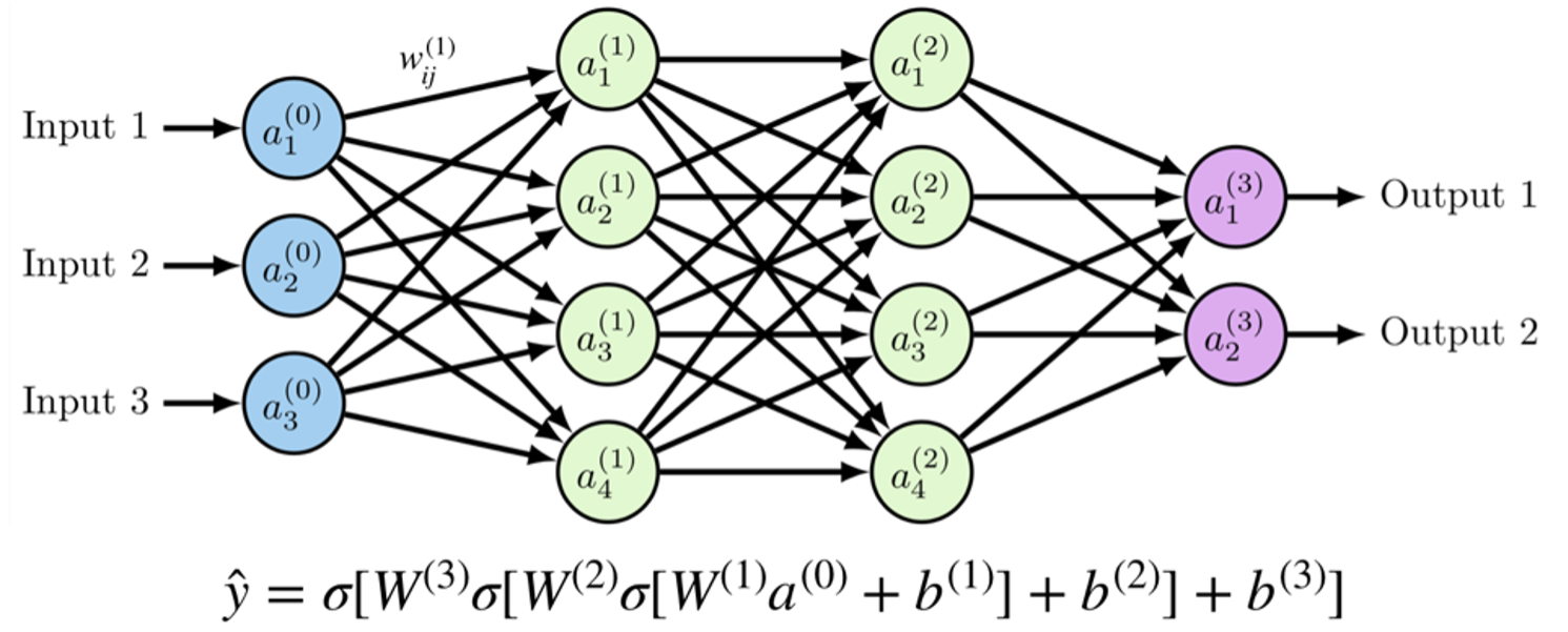
The composition can be seen where the weights outputted from each layer (W1, W2, W3) are the inputs to the next layer, like a loop fed into itself. So, in this case, \(W3 \sigma\) is a function of \(W2 \sigma\) which itself is a function of \(W1 \sigma \).

It's important to walk away with this insight: talking about composition functions is not just an exercise in mathematics, it’s actually the formal way to explain what has been popularly called “modularity” like Lego blocks - the ability to swap in and out different non-linearities, adapt the architecture for different layers, connectivity patterns, apply special blocks, add regularization, normalization, and more, is a beneficial feature of this compositional architecture.

There are a wide variety of design choices in developing a variety of neural networks from recurrent neural networks, convolutional neural networks, autoencoders, transformers, and more, to output the best prediction possible. But in order to output the “best prediction possible”, we need to scan all the possible ways the model could make a prediction.

Optimization helps to search the space of all possible parameters, or weights, used to output a prediction. Weight matrices are called gradients and they serve to guide the learning of the network, to inform how much and in which direction the algorithm needs to fine tune in order to minimize the error between the prediction and the ground-truth. Further, the gradients can be inspected to assess whether the algorithm is learning or not. For example, with a sigmoid activation, the sigmoid function when plotted flattens when close to zero or one. If the gradients are consistently close to zero or one (derivative), we can say they are “saturated”, and the algorithm is not learning.

Loss Functions

As Google Chief Executive Sundar Pichai once said, “It’s not enough to know that an AI model works. We have to know how it works.”

Let's begin with a simple overview of the loss functions that provide optimization algorithms like gradient descent, the feedback they need to update weights and minimize error. Loss or cost functions (often used interchangeably) are used to calculate the error between a ground truth sample and the predicted sample.

The errors calculated are used as a source of feedback during back propagation to optimization algorithms like gradient descent. Typically, we see neural networks optimized to minimize error calculated by the loss function. In other cases, like reinforcement learning, the network is trained to maximize the objective referred to as the reward. Objective functions are described in terms of loss functions. The loss tells the optimization algorithm how successful it has been in outputting the best possible prediction. For example, here is a loss function we will introduce later, called Mean Squared Error:

$$ J (\theta)= \frac{1}{n} \sum_{i=1}^n (y^i - \hat{y^i})2 $$

$$ min_\theta J(\theta)$$

We can use this loss function in a simple example of a minimization objective, which just asks us to find a value of theta that will minimize the loss function. These objective functions can grow increasingly more complicated for different AI algorithms, such as Generative Adversarial Networks where two neural networks must compete against each other and have different objectives.

The Popular Kid: Cross Entropy

In a 2019 interview with Wired, Geoffrey Hinton, the credited “Godfather” of AI and winner of the 2019 Turing Award talked about the notion of surprise:

Once you've got a model, you can say, “How surprising does a model find this data?” You show it some data and you say, “Is that the kind of thing you believe in, or is that surprising?” And you can sort of measure something that says that. And what you'd like to do is have a model, a good model is one that looks at the data and says, “Yeah, yeah, I knew that. It's unsurprising.

Dr. Hinton’s mention of the word “surprise” is intentional and a good segue into loss functions and measuring how algorithms learn. Surprise relates to information entropy, essentially the theory that jump started the field of information theory by Claude Shannon. In a 1948 paper entitled “A Mathematical Theory of Communication”, Shannon lays out information entropy as a measure of information content, having developed this based on his work in cryptography at Bell Labs during World War II.  A very surprising event would rarely happen, and therefore has a very low probability say 2%.   Whereas, an unsurprising event, one that happens frequently, and we know will occur, has a high probability of say 95%. 

For a single event, X we can calculate its entropy as $$ H(P(X=x)) = -log_2 P(X=x)$$ In our example, let’s say a highly probable event is that our alarm will go off in the morning, so $$ -log_2 P(X=0.95) = 0.022$$ whereas an improbable event might be that an airplane will land in our front yard which is 1.698. In machine learning, we seek to measure the expected cross entropy, or the average across all events. We call this the cross-entropy (a combination of softmax regression that generalizes logistic regression into a multi-class problem, with negative log likelihood) of a model Q on the data distribution P, where x is our observations (e.g. events) and p(x) is the distribution of our real ground truth data and q(x) is our distribution of predictions.

$$ H(p,q) = - \sum_x p(x) \log q(x)$$

In Geoff Hinton’s description of an ideal model, he was describing that a correct machine learning model needs to be the least surprised by the unseen data. It should have low entropy or low surprise, close to zero per our alarm clock example. This should occur because the algorithm has mapped all the feature distributions and has achieved good generalization. It “knows” unfamiliar events so well that it can expect them to occur; nothing is surprising. It has essentially minimized the risk by minimizing entropy or surprise of the system. Further, by evaluating the cross entropy of an algorithm, we can understand how much of a model’s errors come from the randomness of the true distribution versus just being incorrect.

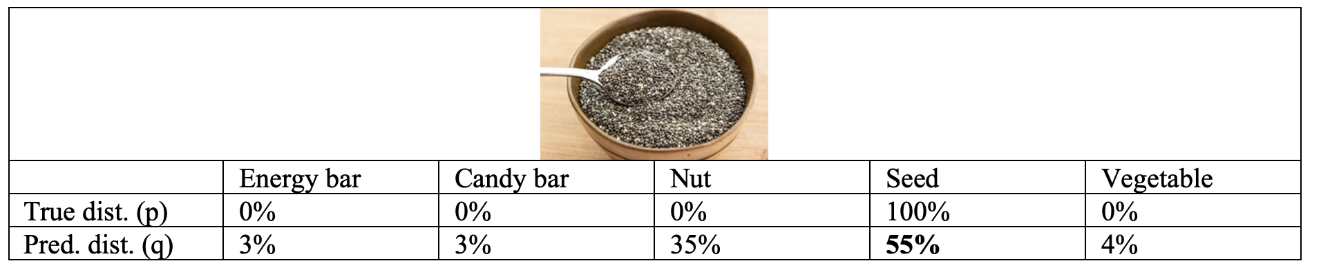
If we had a health food image classifier, we could calculate the cross-entropy loss for how well the model predicts this picture of chia seeds. Our classifier predicts that this is a seed (chia seed) class at 55%. The predicted distribution (q) is provided below. The true distribution (p) shows that across all five food classes (Energy bar, Candy bar, Nut, Seed, Vegetable), the ground-truth for this image being in the "Seed" class is 100%. If we think of this as a one hot vector it would be like \([0, 0, 0, 1, 0]\) - Energy bar: 0%, Candy bar: 0%, Nut: 0%, Seed: 100%, Vegetable: 0%"

$$\text{Cross-entropy loss}: H(p,q) = -\sum_i p_i \log q_i = -1.0 \log(0.55) = 0.259 $$

The closer the cross-entropy value is to 0 means that the predicted distribution is closer to matching the true label distribution (which would be 100% seed not 55% seed). For example, if the prediction was 95%, the cross-entropy loss would be equal to \( -1.0 * \log (0.95) = 0.022\) and for 99% it would be \( -1.0* \log (0.99) = 0.004\). The "surprise" is getting less and less as the model becomes more precise.

Regression Errors - MSE, MAE, RMSE

For regression problems we can use different evaluation measures to assess the performance of the model. We can also use these same functions as loss functions.

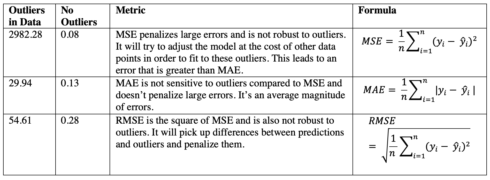
First, let’s take a look at two simple linear regression models. One model has a fairly uniform distribution of data. For this model we see a Mean Squared Error (MSE) of 0.08, Mean Absolute Error (MAE) of 0.13, and Root MSE of 0.28. We might choose to accept the MSE as the evaluation metric of choice to explain how well our model predicted on this dataset.

But in our second model, we see some noticeably unusual values that are above 100. We might consider these as outliers. When we calculate MSE, MAE, and RMSE we can see that each are very different especially MSE at 2982.28 which is much higher than MAE or RMSE.

You may want to approach the dilemma of which metric to use, based on how you are thinking about outliers. Do you expect the data to be noisy, with some outliers here and there, but they mean nothing?  But consider another case. Perhaps these outliers are not mistakes or accidents, but real data points.

Let’s take for example Michael Phelps’ swimming record of wins compared to other swimmers of comparable age and fitness. His record is an outlier, not a mistake. It contains behavioral information that could be important in a model measuring swimming performance. 

If the outliers are important to you and need the model to fit them, then using MSE could be valuable to assess its performance. If the outliers are not important and may be representative of noisy data like intentional breaks in data collection, MAE may be a better metric. For examples of how to deal with outliers including some Python code, check out this post.

References:

1. Janocha, Katarzyna, and Wojciech Marian Czarnecki. "On loss functions for deep neural networks in classification." arXiv preprint arXiv:1702.05659 (2017).
2. https://quebecartificialintelligence.com/academy/
3. https://www.cnet.com/news/google-working-to-fix-ai-bias-problems/
4. https://www.wired.com/story/ai-pioneer-explains-evolution-neural-networks/
5. http://people.math.harvard.edu/~ctm/home/text/others/shannon/entropy/entropy.pdf
6. "https://medium.com/analytics-vidhya/backpropagation-for-dummies-e069410fa585"
7. Bewley, Thomas, Parviz Moin, and Roger Temam. "A method for optimizing feedback control rules for wall-bounded turbulent flows based on control theory." ASME-PUBLICATIONS-FED 237 (1996): 279-286.

FYI - Apologies for some of the imprecision in the mathematical syntax. Unfortunately the ghost.io editor couldn't handle some of my latex expressions. Note that W1 refers to \(W^{(1)}\) and so on.