A Brief Overview of GANs
Introduced by Goodfellow, et al. (Goodfellow) in 2014, a GAN consists of two functions, a generator and a discriminator, which are usually neural networks but can be any differentiable function. GANs are used to map data from one space to another; typically from a generated distribution \(p_g\) to an unknown, true data distribution \(p_{data}\). GANs belong to the family of implicit density models. As such, GANs generate data samples and use these generated data to modify the data-producing model without supplying it an explicit hypothesis (Gui). Doing so allows the GAN to learn high dimensional mappings of complex data like videos, images, and text.
How is GAN Trained?
The generator, G, is a differentiable function represented in the original Goodfellow paper (Goodfellow) as a multi-layer perceptron (MLP). G captures a mapping from noise space to data space and is represented as \(G(z;\theta_g)\) where \(\theta_g\) are the parameters of G's neural network: \(G: z \rightarrow{G(z;\theta_g)}\) (Goodfellow; Skrede). The discriminator, D, is also a differentiable function and maps the input \(x\) to \(D(x,\theta_d)\): \(D: x \rightarrow{D(x;\theta_d)}\). The output of D is a scalar and is the probability that the sample, \(x\) is from the real distribution \(x \sim p_{data}(x)\) notated as \(D(x)\), or from the prior, generated distribution such as Gaussian noise, \(z \sim p_z(z)\), notated as \(D(G(z))\). Both G and D are trained jointly to solve the following objective function, introduced by Goodfellow:
\[\min\limits_{G}\max\limits_{D} V(D,G) = E_{x\sim p_{data}(x)} \log D(x) + E_{z \sim p_z(z)} \log (1 - D(G(z))\]
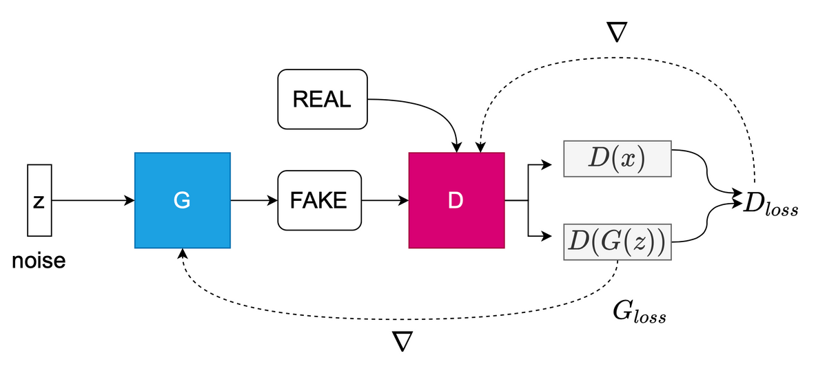
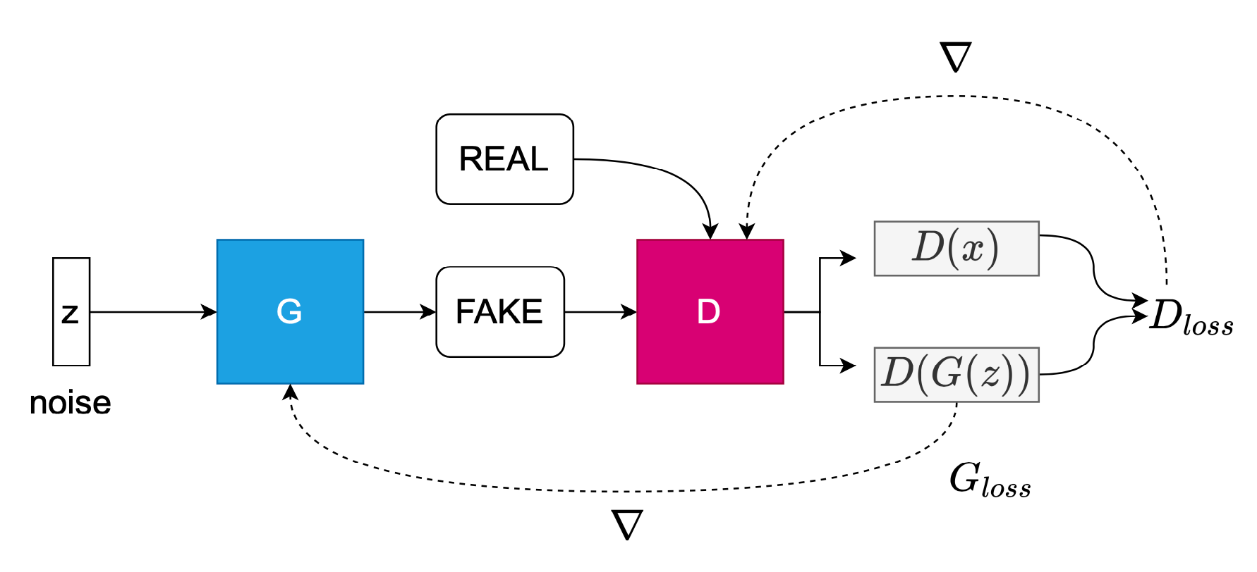
In Figure 1, the discriminator and the generator are pitted against each other, with each cost function optimizing opposing goals. Goodfellow likens this to a zero-sum, minimax game where the sum of all players costs are zero: \(J^{(G)} = -J^{(D)}\). D wants to maximize its probability of predicting the correct label to both the real training data \(p_{data}\) and the fake training data (drawn from the \(p_g\) distribution) as real = 1 and fake = 0, respectively. \(D(x)\) outputs probabilities closer to 1.0 when samples are predicted as real and closer to 0 when samples are predicted as fake. As a result, D tries to force \(D(G(z))\), the probability of the sample as fake, closer to 0. Meanwhile, G is trained to minimize the objective function so that \(D(G(z))\) is close to 1, minimizing \(\log(1 - D(G(z))\). In this way, the D is fooled into believing \(G(z)\) is real. As a result of this duel, the generator can be thought of as a counterfeiter and the discriminator as the police. The generator attempts to fool the police into believing its fake bank notes are real. Here is an easy to understand example of Goodfellow's GAN implemented in PyTorch. Here is the 2016 Tutorial at NeurIPS given by Goodfellow.
Understanding GAN as BCE Loss
We can think of the basic GAN objective in terms of binary cross-entropy (BCE) loss (Saxena; Hong) per \(L_{BCE}(y, \hat{y}) = -y*\log (\hat{y}) - (1 - y)*\log (1 - \hat{y})\). D can be considered as a binary classifier (e.g. sigmoid activation), with a supervised target of 1 for real images and 0 for fake, as indicated earlier. In order to update G's parameters, the generated fake image is passed to the D with a target of real = 1. A forward pass is made through D which calculates the gradient with respect to the fake image. Hence, there are two mini-batches of data passed to D, a real batch and a fake batch. Now, G can use the gradient to update its network and produce more deceptive images.
If we set \(y = 1\) for real data \(x \sim p_{data}(x)\) (x is drawn from true distribution), and set \(\hat{y} = (D(x))\) the real discriminator loss is found via:
\[L_{real}(x) = L_{BCE}(1, (D(x))) = -\log (D(x))\]
If we set \(y = 0\) for fake data \(x \sim p_g\) (x is drawn from fake distribution), and set \(\hat{y} = D(G(z))\) then we see the fake discriminator loss in:
\[L_{fake}(x) = L_{BCE}(0, (D(G(z))) = -\log (1 - (D(G(z)))\]
The total discriminator loss is a summation of the \(L_{real}(x)\) and \(L_{fake}(x)\), and gradient ascent is applied to train D in:
\[\max\limits_{D}E_{x\sim p_{data}(x)} \log D(x) + E_{z \sim p_z(z)} \log (1 - D(G(z))\]
For the generator, \(y = 0\) for the fake label, and the loss is maximized in:
\[L_{G}(z) = L_{BCE}(0, (D(G(z)))) = -(1 - \log (D(G(z))))\]
Gradient descent is then applied on the generator in:
\[\min\limits_{G} E_{z \sim p_z(z)} \log (1 - D(G(z))\]
However, when G is of the form \(\log (1 - D(G(z))\), its gradients are flat at values where \(D(G(z))\) has lower probability values from 0.0 - 0.5 per the blue curve in Figure 2. This is a sign of vanishing gradients notorious in GANs for instability. It means that G cannot learn from the gradients of D, particularly when G's samples are poor (the lower probability regions). However, the gradients are steep when \(D(G(z))\) is closer to 1.0. Herein lies the reason why in practice, gradient ascent is used to maximize G, maximizing the term \(-\log(D(G(z))\), instead of \(\log (1 - D(G(z))\) per \(\max\limits_{G}E_{z \sim p_z(z)} -\log D(G(z)))\).
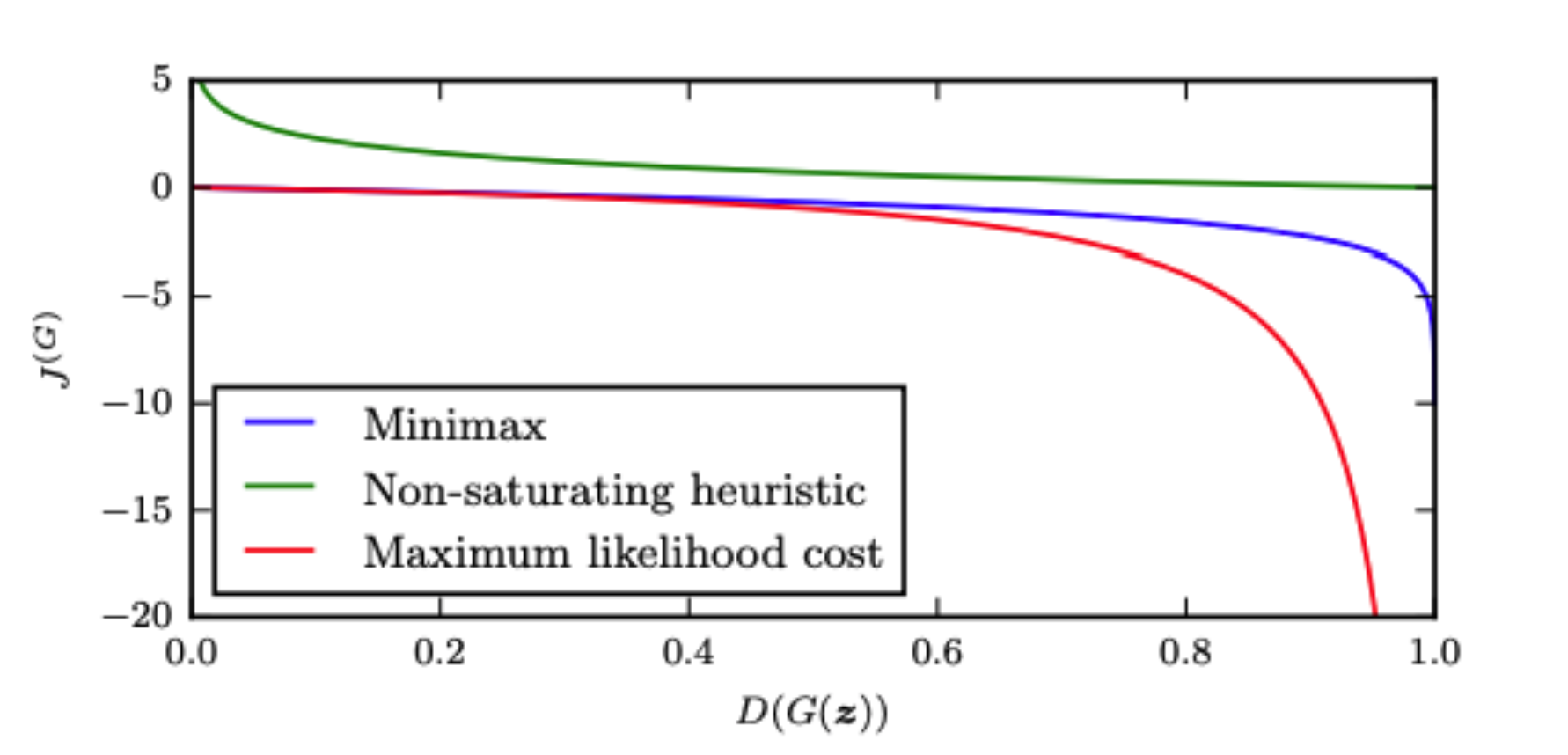
The shape of the the new function (\(-\log(D(G(z))\)) then allows for gradients in the regions closer to zero to have curvature, allowing G to learn. This is called the "non-saturating heuristic" (Goodfellow; Gui; Skrede) per the green curve in Figure 2. This high gradient signal gives the generator a "fighting chance". Such gradients are beneficial for G early in training when the fake samples are obviously different than real data. In this early phase of training, D has a much easier job than G, easily descending to outputs of 0 predicting each sample \(D(G(z))\) to be fake.
When will GAN converge?
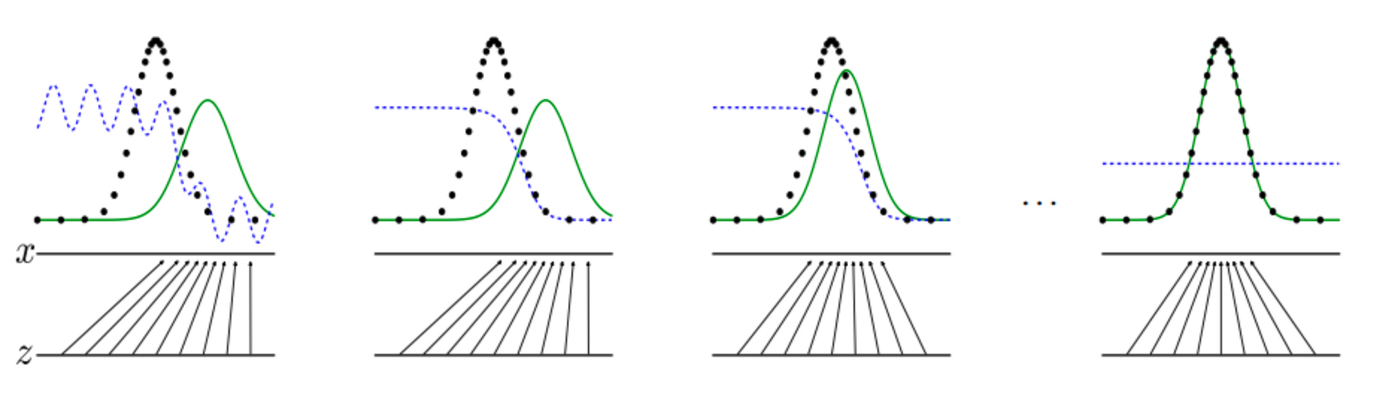
The global minimum of the training criterion, \(C(G) = \max\limits_{D} V(G,D)\) can only be achieved if and only if \(p_{data} = p_g\) as explained in Figure 3, where both distributions have reached a Nash Equilibrium (due to the minimax game theory scenario). Given a fixed G, D converges to an optimal discriminator per below. As a result, D estimates the ratio of two probability densities (Wang).
\[D(x)^* = \frac{p_{data}(x)}{p_{data}(x) + p_g(x)} = \frac{1}{2}\]
Goodfellow shows this by taking the derivative of the training objective (in the form binary cross-entropy loss), setting the training objective to zero, and plugging in \(p_{data} = p_g\). By substituting \(D(x)^*\frac{1}{2}\) into the cost function \(V(D,G)\) we find that \(V(D^*, G) = -\log(4)\). However, when the data distributions between real and fake are not the same, \(p_{data} \neq p_g\), the global minimum, \(C(G)\) has additional Kullback-Leibler (KL)-divergence terms shown below. But rearranging the below shows that the two KL terms can be represented as the Jenson-Shannon (JS) divergence \(JSD(p_{data} \Vert p_g)\) between \(p_g\) and \(p_{data}\).
\[C(G) = -\log(4) + \textcolor{red}{KL(p_{data} \Vert \frac{p_{data} + p_g}{2}) + KL(p_g\Vert\frac{p_{data} + p_g}{2}})\]
The entire JSD term, below, goes to zero if \(p_{data} = p_g\) which occurs when \(D(x)^* = \frac{1}{2}\).
\[C(G) = -\log(4) + \textcolor{red}{2*JSD(p_{data} \Vert p_g)}\]
Mode Collapse
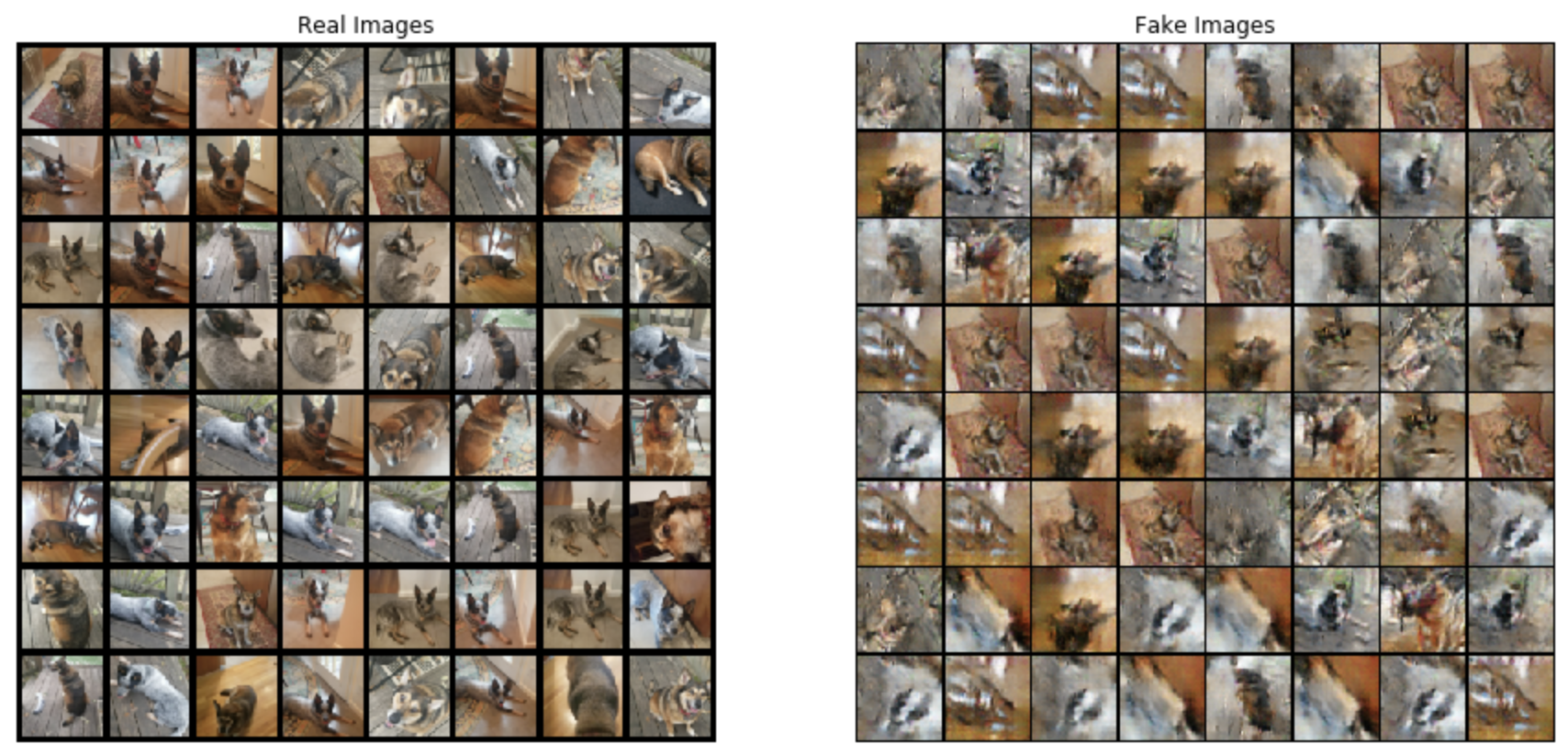
These mathematical principles the occurrence of "mode collapse", a major challenge of GANs. In mode collapse, the generator learns to produce samples from a few number of modes. Symptoms include generation of images with low diversity, having been drawn from the same distribution repeatedly.
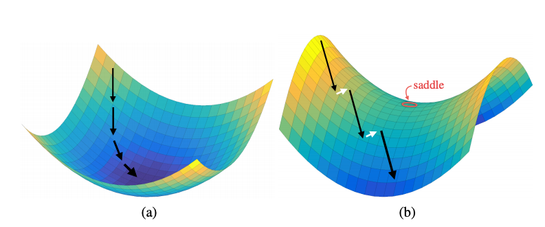
Recall the objective function in Goodfellow's GAN. With \(\min\limits_{G}\max\limits_{D} V(D,G)\), D is updated with gradient ascent and G is updated with gradient descent. Another way to think about the steps taken by the GAN algorithm during training is minimization in an outer loop by G and maximization in an inner loop by D (Goodfellow). As we have already seen, this means that the discriminator and generator alternate training steps, where in the outer loop G minimizes \(\max\limits_{D}\) (Goodfellow). Ultimately G and D converge to a saddle point shown in Figure 4 where \(p_{data} = p_g\), the maximum of D and the minimum of G. Mode collapse occurs in the journey to reach this saddle point. In Figure 4 (b), Yadav et al. (Yadav) show how adversarial training is challenging because if either the generator or discriminator out powers the other, the gradient will "slide off" the loss surface. This leads to instability and a sudden collapse of the network - e.g. mode collapse.
In the traditional model previously introduced, the GAN seeks parameters to maximize the likelihood of training data, \(\min\limits_{G}\max\limits_{D} V(D,G)\). By minimizing the KL Divergence, the GAN will generate across multiple modes of \(p_{data}\), but at the same time generate artifacts and images from unseen distributions. If the GAN is trained to use reverse KL divergence meaning how much to distort \(p_g\) into \(p_{data}\), a "mode seeking" behavior will occur leading to mode collapse (Nguyen). In Unrolled GAN, the authors show how a standard GAN causes the generator to rotate through different modes, but never converge to the fixed target distribution, and assigns probability mass to only one data mode at a time (Metz).
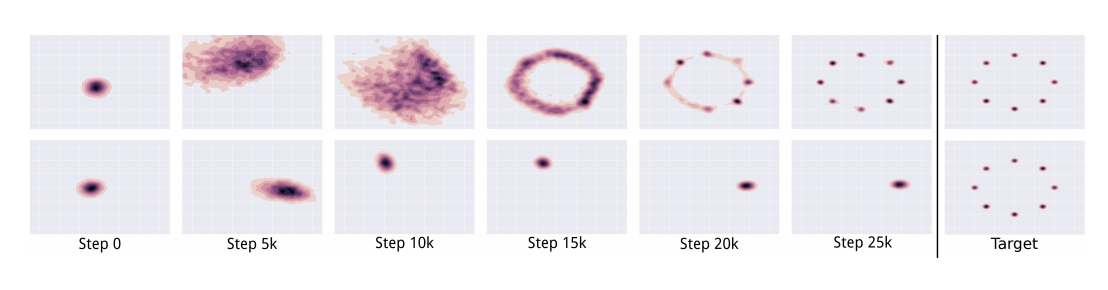
With mode seeking, the GAN may prefer a majority mode as explained by Che et al. and shown in Figure 5. In this scenario, the generator produces few samples that will improve the distributions around the minority modes (Che). This is a phenomenon called "missing modes" and can occur even if modes are available in the data (Che, Gui). The generator ends up producing low-diversity samples that are repetitive and "safe". Safe in the sense that the generator is penalized more heavily for outputting structurally inaccurate samples, as opposed to ones that are somewhat realistic. Hence, it outputs, with low diversity the same samples over and over again, opting for realism over diversity. It never spreads probability mass across all modes.
How to Mitigate it?
A variety of objective functions have been developed to stabilize GAN and thereby minimize mode collapse. Notable contributions include: 1) Wasserstein GAN (Arjovsky) which seeks to minimize the Earth Mover's distance as an alternative to f-divergence (e.g. JS divergence), 2) LSGAN (Mao) that uses Mean Squared Error (MSE) to penalize fake samples that are far away from the real and fake decision boundary, and 3) Unrolled GAN (Metz) in which the generator looks several steps ahead for how the discriminator may optimize its output thereby discouraging it from producing an output at the same local mode. Other techniques include: 1) One-sided label smoothing that makes it more difficult for the discriminator to learn by converting the real = 1 label to real = 0.9. (Soumith), 2) Increasing learning capacity of the GAN through StackGAN (Zhang) that breaks up the learning into smaller stages, 3) Using deep features extracted from pretrained networks like VGG16 as means of optimizing perceptual similarity (Zhang, Isola, et al), and 4) "Jacobian Clamping", which is a form of regularization to reduce inter-run variance and constrain the conditioning of the Jacobian (Odena). It is worthwhile to briefly discuss \textbf{WSGAN} as a major contribution towards stability.
To begin, the training objective using JS divergence and log likelihoods in the original GAN, work when the two distributions of \(p_{data}\) and \(p_g\) overlap, making JS divergence equal to 0. But in image modeling, it's not typical early in training, for the real images \(p_{data}\) to lie on the same high-dimensional space (e.g. manifold) as the noisy images \(p_g\) (Sønderby). As a result, if \(p_{data}\) and \(p_g\) do not overlap, it will cause the gradients from the JS divergence to be flat everywhere, and the log-likelihood and KL divergence to be infinite. Essentially, the generator will be incapable of learning, going back to the use of the non-saturating heuristic in Figure 4.
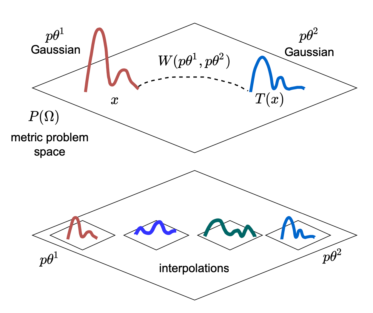
To counteract this and support the generator with gradients, the Wasserstein GAN uses the Earth Mover's Distance (EM) (aka Wasserstein-1 distance) instead of f-divergences. EM distance calculates how far apart \(p_{data}\) is from \(p_g\). EM distance comes from the field of optimal transport theory, where algorithms are used to compare the distances between different probability measures. The EM distance is not so much a function, but rather a distance calculation between metrics of two probability distributions (Cuturi). We can think of EM distance (which I'll refer to moving forward as the Wasserstein Distance) as the cost of bringing sand from one point of mass \(x\) to another point of mass \(T(x)\), where we want to minimize the distance traveled and the energy needed to carry the sand over. The Wasserstein Metric, below, describes the distance to move the mass at point \(x\) to point \(T(x)\). Along the way, the distributions are interpolated to minimize the cost function \(\int_\Omega D(x,T(x))\mu(dx)\).
\[W(\mu, v) \coloneqq \min\limits_{x,y} E\|{x-y}\|\]
\[W(P, Q) = \sup \limits_{\|{f}\| L\leq{1}} E_{x\sim{P}}[f(x)] - E_{x\sim{Q}} f(x)\]
But, the EM distance is not differentiable. As a result, there is an alternative definition that can be optimized. Notice how in Figure 6, we show the movement of one data point, \(x\) to another, \(T(x)\). Kontorovich was able to relax the Wasserstein Distance and change the assumptions to move it not from one discrete point to another, but rather one \emph{probabilistic distribution to another}. This is shown in the Wasserstein distance equation above where Gaussian \(P = p\theta^1\), Gaussian \(Q = p\theta^2\), \(x = x\), \(y = T(x)\), to match terms in Figure 6. These functions f(x) must be 1-Lipschitz continuous. What this essentially means is that the function needs to be differentiable everywhere and that the absolute value of the derivative (i.e. the magnitude of the rate of change), is bounded to be above 1. Implementing WGAN requires removing the logarithms from the objective function and clipping weights to enforce the 1-Lipschitz continuity for the gradient.
Limitations and Extensions
Per the famous adage by George Box,"All models are wrong, but some models are useful, also known as the "No Free Lunch Theorem". Assumptions that work to generate data from one domain may not be applicable to another. Many GANs are custom built for their respective task whereby controlling mode collapse in one may not be applicable to another. Further, there are trade-offs when it comes to practical use. For example, the original WGAN implementation requires tuning the sensitive weight clipping parameter (Saxena; Arjovsky), LSGAN prevents mode collapse but does not actually increase the variety of modes (Mao; Saxena), and many other approaches have high computational complexity like Unrolled GAN (Mao; Saxena)
Extensions of existing approaches include designing loss functions towards objectives that are target and application-specific. Both Olut (Olut)and Ledig (Ledig) note that the ideal loss function depends on the application. For example Olut, et al. develops a loss function to reproduce vascularities in images focused on the direction of texture of MR Angiography images (Olut). Ledig, et al. also points out that loss functions that hallucinate fine detail may be inappropriate for surveillance or medical applications (Ledig). Additional extensions include integrating side information that reflects the modality of the target domain such as text, class labels, or semantic maps to condition the generator (Odena). Perceptual loss functions such as LPIPS use feature vectors extracted from a pretrained network like VGG19 (Zhang, Isola, et al) helps in cases of super resolution, whereas applying attention (Zhang) can guide feature maps, and implementing different architectures such as an auto-encoder for a discriminator in BEGAN (Berthelot) or multiple GANs in StackGAN (Zhang) may improve stability and modeling capacity.
References
Goodfellow, Ian J., et al. "Generative adversarial networks." arXiv preprint arXiv:1406.2661 (2014).
Chintala Soumith. How to train a gan? tips and tricks to make gans work, 2016.
Marco Cuturi. Regularized wasserstein distances minimum kantorovich estimators, 2017. https://www.youtube.com/watch?v=T9O6T5WHdC8&t=656s