What is AutoGAN?

AutoGAN is an architecture search strategy developed by Gong, et al. in 2019 to find the most optimal Generator network architecture using reinforcement learning, trained to generate images from CIFAR-10 and STL-10. To understand how AutoGAN works requires an understanding of the basics of Neural Architecture Search (NAS). This post is an overview of both methods, per:
- Zoph, Barret, and Quoc V. Le. "Neural architecture search with reinforcement learning." arXiv preprint arXiv:1611.01578 (2016).
- Gong, Xinyu, et al. "Autogan: Neural architecture search for generative adversarial networks." Proceedings of the IEEE International Conference on Computer Vision. 2019.
- Here's the implementation of AutoGAN which is in PyTorch: https://github.com/TAMU-VITA/AutoGAN
The Motivation
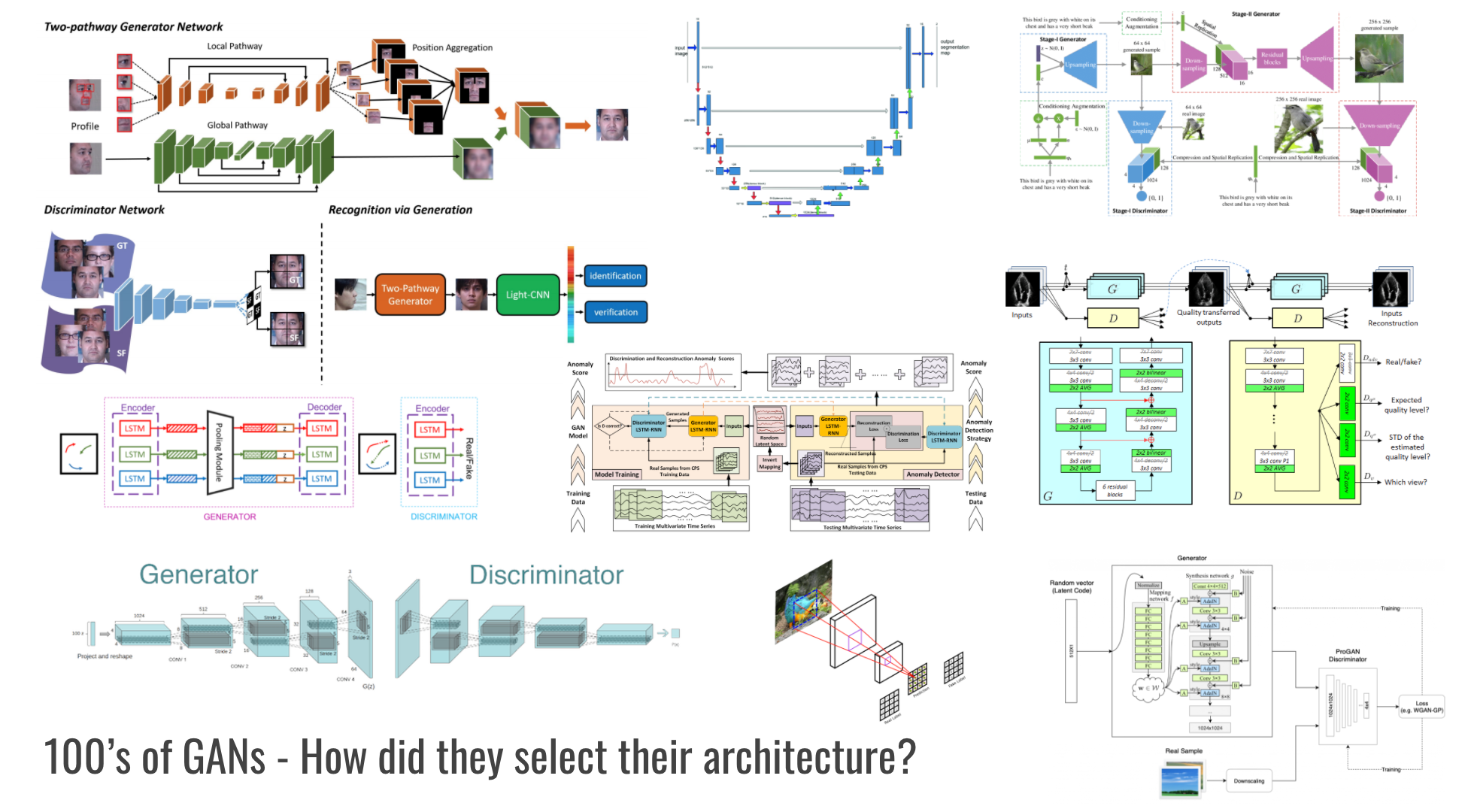
There are hundreds of GANs! If you navigate to Avinash's GAN Zoo at https://github.com/hindupuravinash/the-gan-zoo, he lists a variety of GANs designed for various domain-specific tasks, some of them more generalizable and cross-domain than other (i.e. WGAN, CycleGAN, pix2pix, DCGAN). Regardless, there are many choices for your domain - from high definition faces, natural scenes, to biomedical images.
Much of this is developed by years of research, technical acumen, and hand-crafted knowledge.
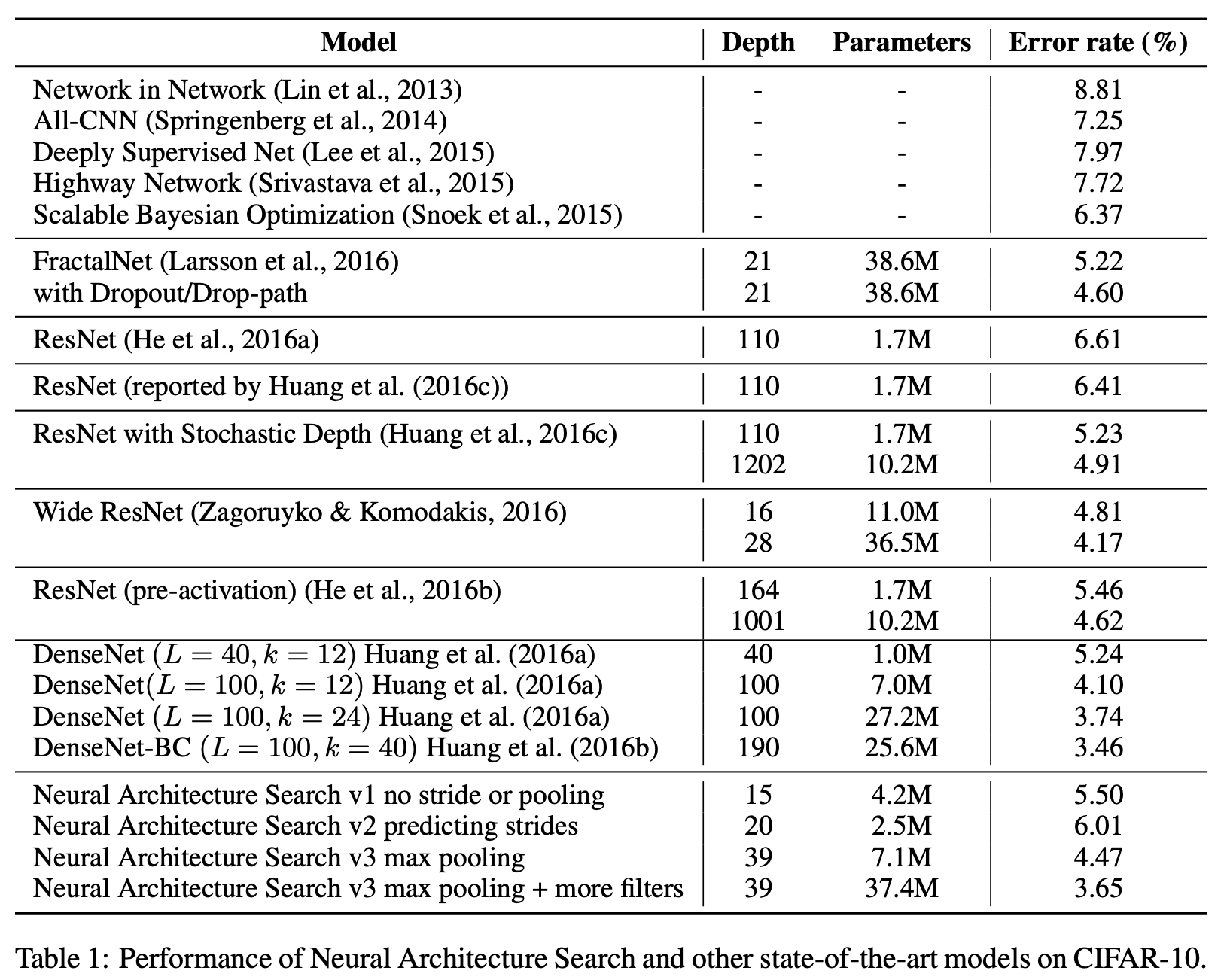
Is there an automatic way to develop these GAN architectures? This is what Neural Architecture Search (NAS) attempts to do. Using NAS, the authors found that it can design several architectures including convolutional neural networks (CNNs) and recurrent neural networks (RNNs) competitive to some of the best performing models on CIFAR-10 and the Penn Treebank, respectively. For example, the best NAS searched architecture was a CNN using max pooling that consisted of 37.4M parameters with a 3.65 error rate on CIFAR-10, compared to DenseNet-BC (Huang et al 2016 at 3.46). The long-short term memory (LSTM) cell found by NAS outperforms other RNNs on the Penn Treebank Task, such as recurrent highway networks by Zilly et al. (66.0 test perplexity) and Inan et al VD-LSTM (68.5 perplexity), with a 62.4 test perplexity.
Neural Architecture Search (NAS)
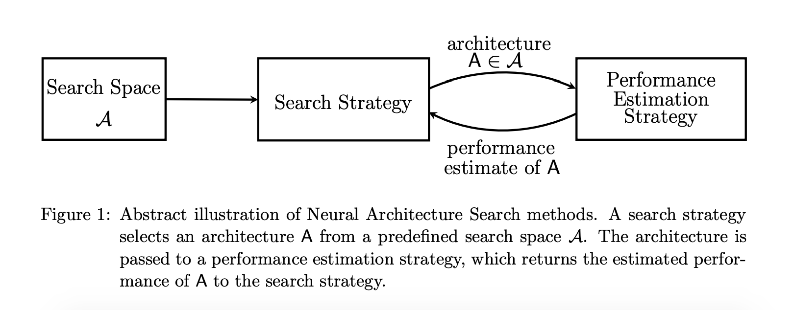
Before digging into the NAS paper, I found a survey paper by Elksen et al. entitled Neural Architecture Search: A Survey. Elksen reviews NAS methods in addition to Zoph & Le's, and presents NAS as a method with three components - 1) the configurations for which a neural network architecture will be searched (Search Space) to generate a candidate architecture, A, followed by 2) a search strategy to optimize the network such as Bayesian optimization or reinforcement learning (RL), and then 3) an estimate, not an exact, measure of the performance of A that can be conducted in a reduced manner such as on a subset of validation data, for a fewer number of training epochs and more, in an effort to minimize GPU training time since the NAS process can take a very long time.
We will see in the AutoGAN paper how they use a proxy training task of a discovered Generator architecture trained from scratch for 30 epochs to evaluate its performance (the Inception Score, which I explain later).
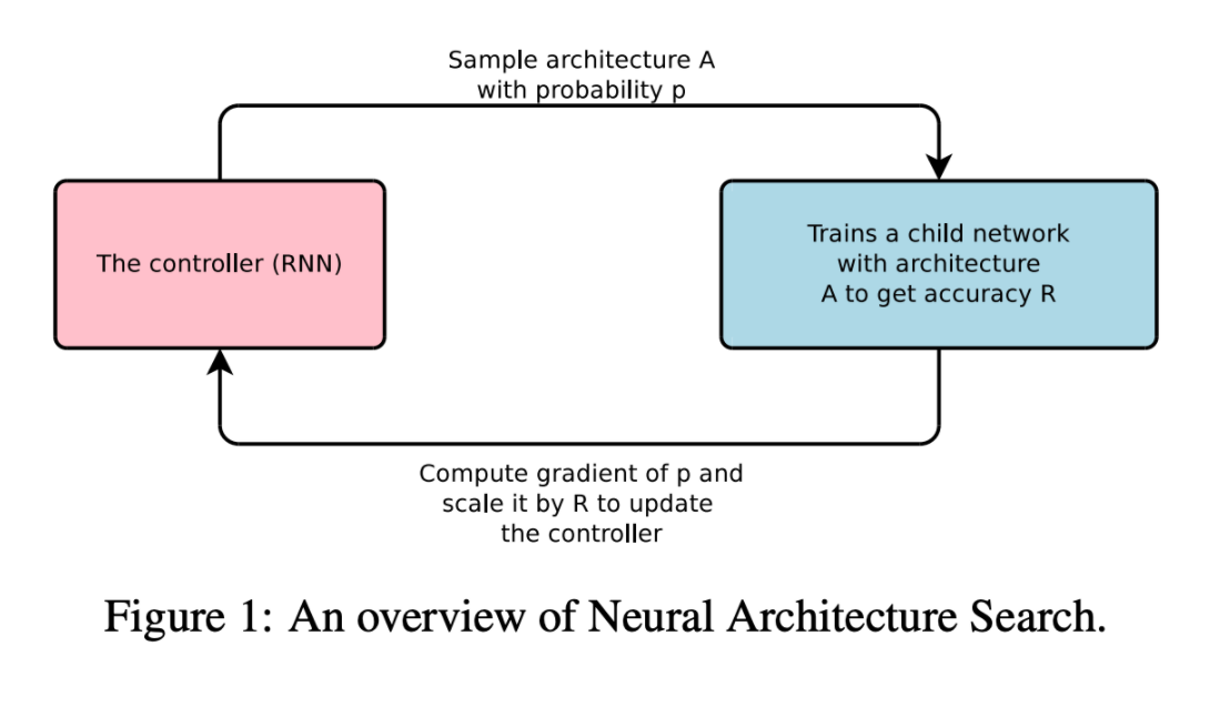
NAS was introduced by Zoph and Le from Google Brain in February 2017 and is a gradient-based method for finding good architectures. It consists of what they call a "Controller" which is a recurrent neural network (RNN) that generates candidate neural network architectures based on a string of hyperparameters. A neural network (the child) is trained using one of the candidate architectures and its validation accuracy on an image classification task (e.g. CIFAR-10) is calculated. Reinforcement learning is used to maximize the expected accuracy R. Gradients are updated for the controller, and it begins again.
We know that a RNN per Chris Olah's depiction below, are used for a variety of one-to-many, many-to-one, and many-to-many (seq2seq) tasks like text classification, language generation, and machine translation. Sequence like inputs and outputs are the data IO that RNNs excel at.
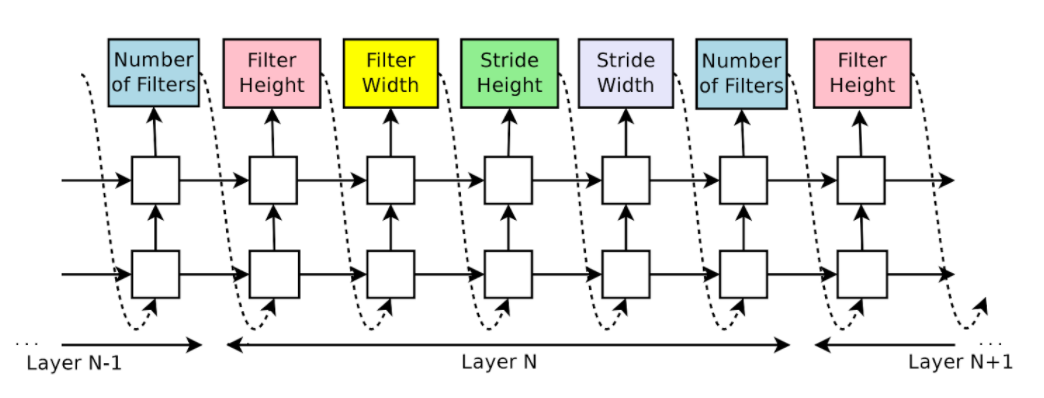
RNNs can be used to generate architectural hyperparameters of neural networks such as the number of filters for each convolutional layer, the filter height, width, stride, etc. Zoph and Le observed that the structure and connectivity of neural networks can be specified by a variable-length (e.g. any length) string, outputted by the RNN much like a string of characters, terms, and values in a one-to-many or many-to-many sequence.
They go on to cite some related work that might come to mind when "searching model architectures" comes to mind. These include methods like Bergstra et al's hyperparameter optimization which Zoph & Le argue is difficult in generating a variable-length configuration that specifies the structure and connectivity of a network and work better with an initial model, in addition to Mendoza et al's Bayesian optimization that Zoph & Le say are less flexible and generic. They also mention the flexibility of neuro-evolution algorithms (like Stanley et al's 2009 HyperNEAT algorithm) for creating novel architectures, but argue that practically they are slow and rely on heuristics. Zoph & Le center towards two schools of thought, one is to search for hyperparameters in an auto-regressive manner, meaning that the controller predicts hyperparameters one a time, conditioned on previous predictions. This idea is borrowed from the decoder in end-to-end sequence to sequence learning which was also co-written by Le, back in 2014 (Sutskever et al., 2014). They also build their idea based on reinforcement learning to use a neural network to learn the gradient descent updates for another network (Andrychowicz et al 2016) and use reinforcement learning to update policies for another network (Li & Malik, 2016).
How it works
There are plenty of complexities in the NAS paper, but here is my general high level overview of the main "steps" involved with the search process.
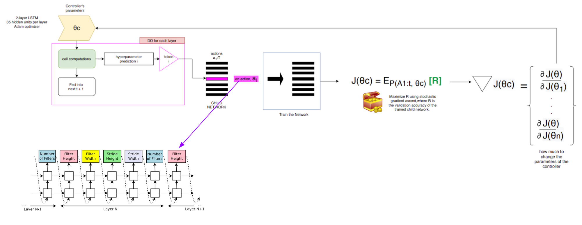
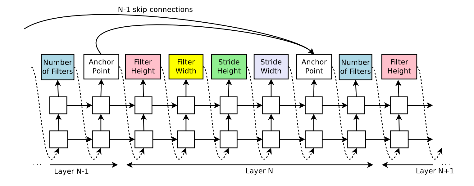
There's a cell computation step, where for each layer of the Controller, it predicts the hyperparameters through a series of RNN cell computations. Next, the child network is trained and the policy gradient optimized. Third, the controller is updated. In the diagram below, theta is the Controller's (RNN) parameters. The hyperparameters predicted at the time step, t, is a token. That token can be considered an action among a list of actions a1:T (the first action to T time-step actions). The network is trained and its validation accuracy used as the reward, R. We want to maximize J (e.g the Controller's parameters gradients) by maximizing the expected (E_P) reward using stochastic gradient ascent. The Controller's parameters are then updated:

The cell computations in my opinion, are the trickiest to understand. Message me if I got this wrong and I can update on my end. These cells may also be interpreted as "motifs" per Elsken et al. versus entire neural network architectures. Architectures are then built by stacking these motifs. Elksen et al. note that this search strategy of finding optimal combination of cells that allow for Zoph & Le to use them for a variety of tasks as we will see later including image classification to language modeling.
I traced the computation steps in Zoph & Le's figure of "an example of a recurrent cell constructed from a tree that has two leaf nodes (base 2) and one internal node. Left: the tree that defines the computation steps to be predicted by the controller. Center: an example set of predictions made by the controller for each computation step in the tree. Right: the computation graph of the current cell constructed from example predictions of the controller." So, as the caption indicated, you can see that the middle blocks is one of any number of predictions a Controller can make. Each RNN in this example has 2 base leaf nodes indicated by Tree Index 0 and Tree Index 1. Both feed into computing Tree Index 2. In this sample computation, we can see that Index 0 is computed as a function of a relu activation with the previous cell state, c_{t-1}. Index 1 is computed as the element-wise multiplicative function of the current input, x_t and the previous hidden state, h_{t-1}. The Index 2 takes the sigmoid activation of the element-wise multiplicative product of both. Note, all these example formulae are provided in the paper.
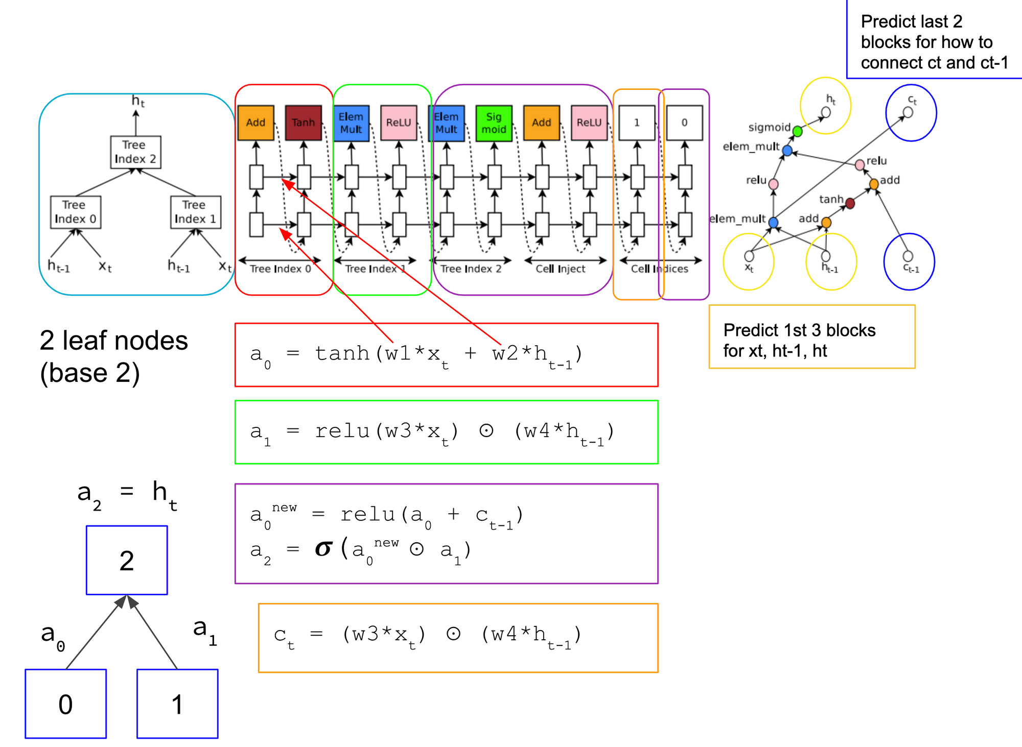
The Controller may also propose skip connections as seen in Residual Nets (He, 2016). NAS adds anchor points at each layer and appears to be specified in the cell computation stage, creating a more complex search space. Being new to reinforcement learning, I found its application for NAS to be very intuitive. Lilian Weng from OpenAI provides a great overview of policy gradient algorithms that explains REINFORCE in addition to several more. First, NAS wants to maximize the reward, R which as we recall is the validation accuracy from the trained child network. e.g 0.98. Since R is non-differentiable, NAS uses the REINFORCE rule from Williams (1992) (see page 9) to iteratively updated the parameters of the Controller, thereby training the RNN.
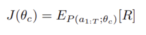
Second, NAS will need to optimize the policy gradient objective, J, for the parameters θc of the Controller (RNN) which is implemented via gradient ascent.
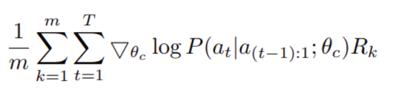
Third, this means that NAS averages over all the actions, a, for each timestep, t, over each state (e.g. child network). To me, this says "the probability to use hyperparameter a, for this m, child network, at timestep t".
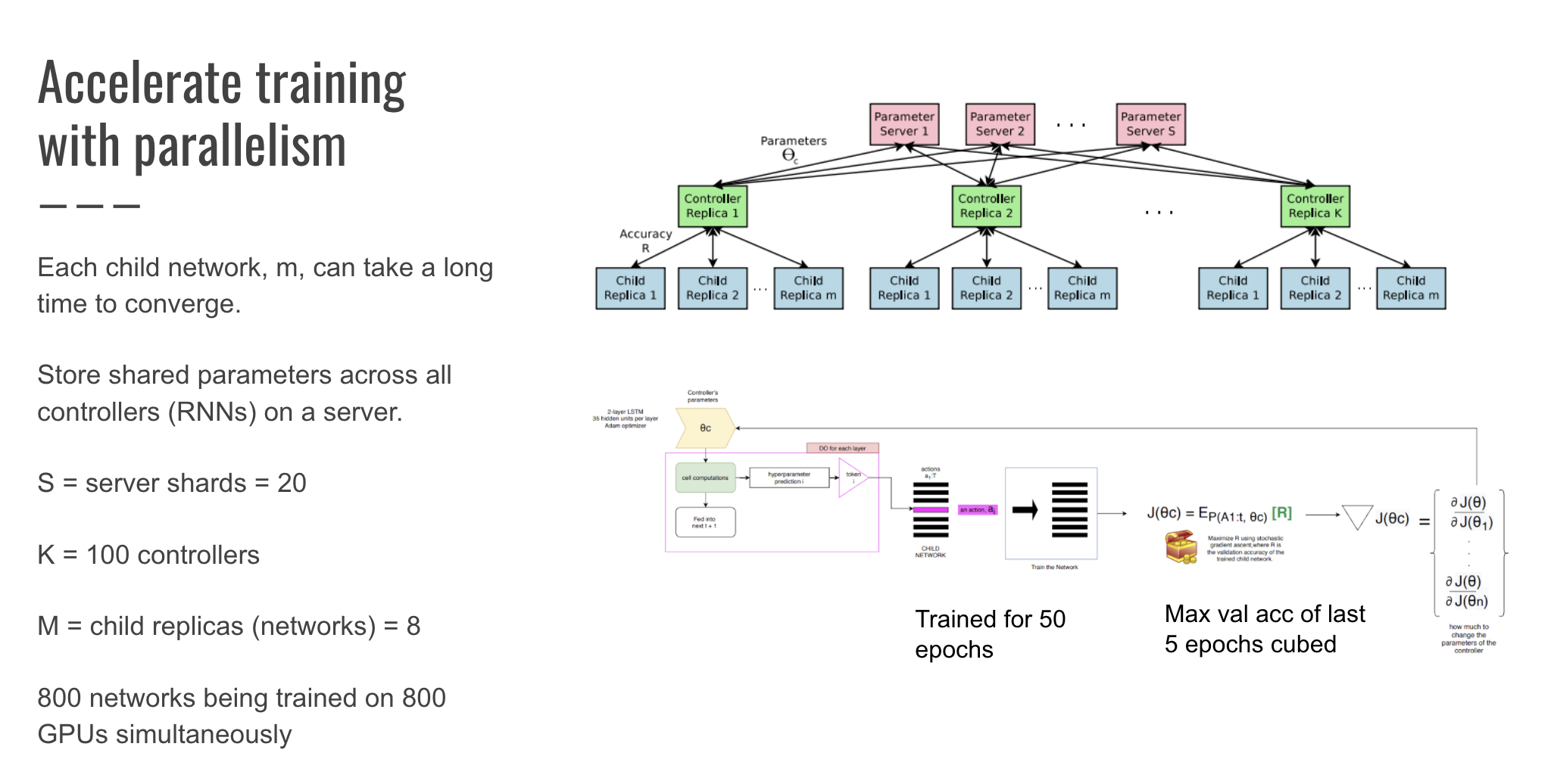
Here's where I paused and realized that NAS seems to be the Cadillac (um, Tesla) of training methods, since I don't possess 800 GPUs. In NAS, Zophe & Le state that each gradient update to the Controller parameters (theta_c) correspond to training one child network to convergence. This can take a long time! As a result, training is distributed. Per the training details, there is a parameter server of 20 shards that store the shared parameters for 100 Controller replicas. Each Controller samples 8 different child architectures that are trained in parallel. The Controller collects the gradients from a minibatch of 8 architectures at convergence and sends these gradients back to the parameter server to update the weights across all the Controllers.
Training
CIFAR-10 training details:
- Controller is a two-layer LSTM with 35 hidden units per layer.
- Trained with Adam optimizer, learning rate of 0.0006
- Weights of each Controller are initialized uniformly between -0.08 and 0.08
- Shards, S = 20; Controller replicas K = 100, m child replicas = 8, total of 800 networks being trained on 800 GPUs simultaneously
- Child network trained for 50 epochs
- Reward, R, is maximum validation accuracy of the last 5 epochs^3
- Validation set = 5000 examples randomly sampled from training set
- Training set = 45,000 images
- Child network trained with: Momentum Optimizer, learning rate 0.1, decay of 1e-4, momentum of 0.9, Nesterov Momentum
- Controller increases depth by 2 for the child network every 1,600 samples starting at 6 layers
The controller trained 12,800 architectures, leading to three top architectures with the best validation accuracy:
- NAS v1 no stride or pooling, depth 15, 4.2M params, 5.50% error rate
- NAS v2 predicting strides, depth 20, 2.5M params, 6.01% error rate
- NAS v3 max pooling, depth 39, 7.1M params, 4.47% error rate
- NAS v3 max pooling + more filters, depth 39, 37.4M params, 3.65% error rate
Discovered Architecture
NAS v3 max pooling + more filters was competitive to DenseNet-BC by Huang et al with a depth of 190 and 25.6M params at an error of 3.46%.
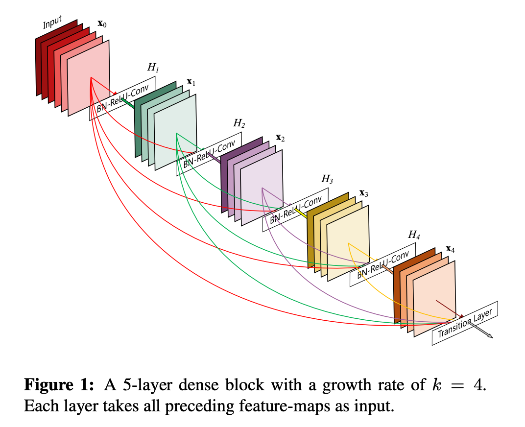
Below is an illustration by Huang et. al of a dense block for DenseNet-BC (k=40). Per Huang et al., Dense blocks, below, use dense connectivity similar to skip connections - direct connections can happen from any layer to all following layers.
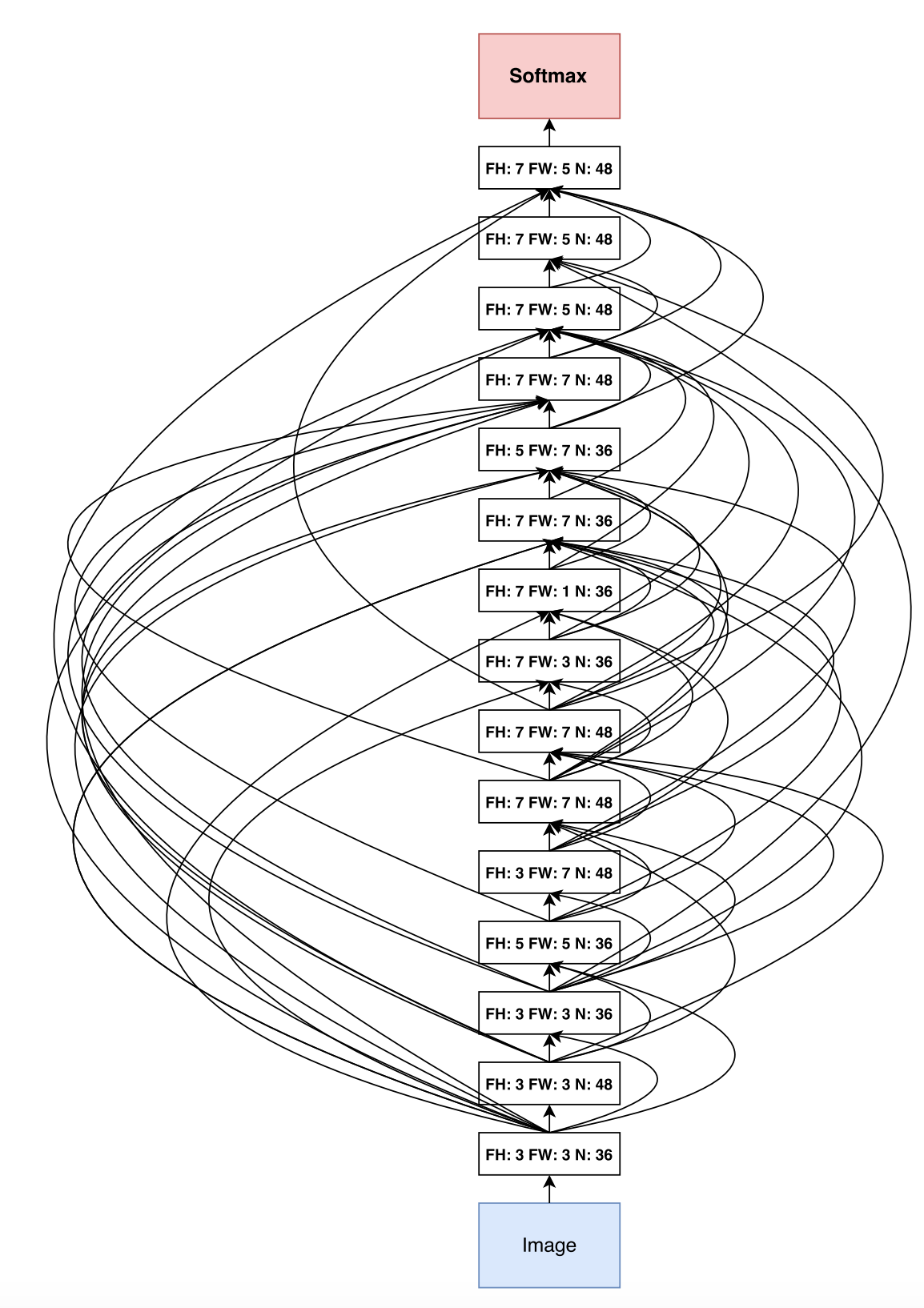
Below is the discovered convolutional architecture by Zoph & Le. Do we see any similarities between it and the higher scoring dense block design above? One thing are the similar "any to any after" skip connections.
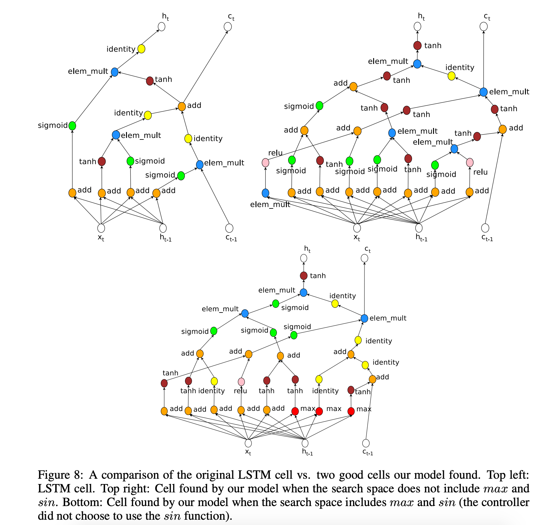
Also Zoph & Le present their discovered cell combinations:
AutoGAN
So now that we understand a few principles of NAS, how about applying this directly to searching for a GAN architecture? Well, there is where Gong et al., come into play. They tell us, whoa, slow down for a minute. Just because NAS's search strategy found an optimum convolutional architecture, doesn't mean it can be applied to GANs, mainly because GANs in themselves are a sensitive bunch -

GANs are sensitive to non-convergence, mode collapse, and sensitivity to hyperparameters, and validation accuracy is not a straight-forward reward policy to use for GANs. Therefore they develop a NAS search strategy specific for discovering an optimum Generator (not Discriminator) architecture. Their method is similar to NAS where there is a RNN controller to guide the search, and they also use REINFORCE policy for RL training, where the Inception Score (IS) is the reward not the validation accuracy. The authors also mention that details about how to grow the Discriminator would be included in the supplementary materials, however, I don't think the version of the paper I have has this supplementary material. As a result, I'm unable to review how the Discriminator was grown.
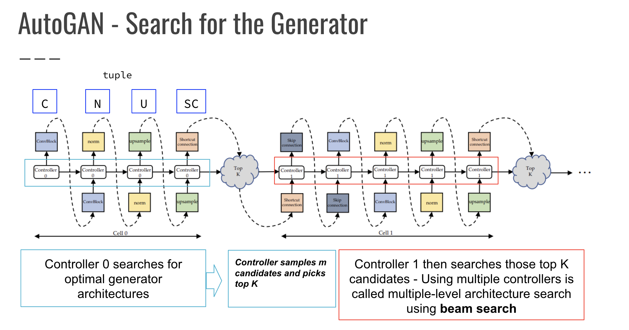
Here, AutoGAN searches for the Generator architecture. A Generator can be composed of many cells. A different Controller is used for the search step of each cell. A search space for a Generator cell consists of a tuple of a convolutional block (C), normalization block (N), upsampling block (U), and shortcut (SC) which is a binary value. Remember, these blocks are similar to "motifs", or design patterns. The Controller searches and then samples the m candidates and picks the top K. Another Controller then searches those top K candidates using something they call a "multi-level architecture search" using beam search:
MLAS performs the search in multiple stages, in a bottom-up sequential fashion, with beam search.
Beam Search, per Sabuncuoglu and Bayiz (1999):
Beam Search is a heuristic method for solving optimization problems. It is an adaptation of the branch and bound method in which only some nodes are evaluated in the search tree. At any level, only the promising nodes are kept for further branching and remaining nodes are pruned off permanently.
My interpretation of MLAS, which may be mistaken so please contact me if I'm incorrect, appears to do with the training methodology of progressively growing a GAN in the ProGAN paper by NVIDIA which the authors cite.
Without progressive growing, all layers of the generator and discriminator are tasked with simultaneously finding succinct intermediate representations for both the large-scale variation and the small-scale detail. With progressive growing, however, the existing low-resolution layers are likely to have already converged early on, so the networks are only tasked with refining the representations by increasingly smaller-scale effects as new layers are introduced.
In addition to Chenxi et al. in Progressive Neural Architecture Search, where the goal is to search for a set of cells or parts of a CNN like blocks, as opposed to finding an entire CNN architecture all at once.
sequential model-based optimization (SMBO) strategy, in which we search for structures in order of increasing complexity, while simultaneously learning a surrogate model to guide the search through structure space
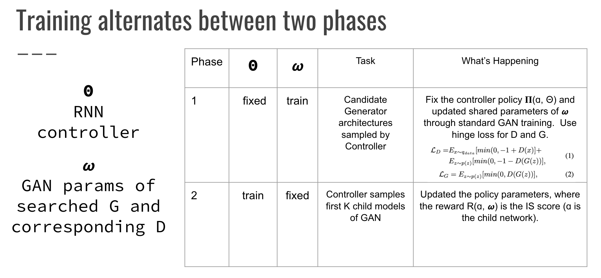
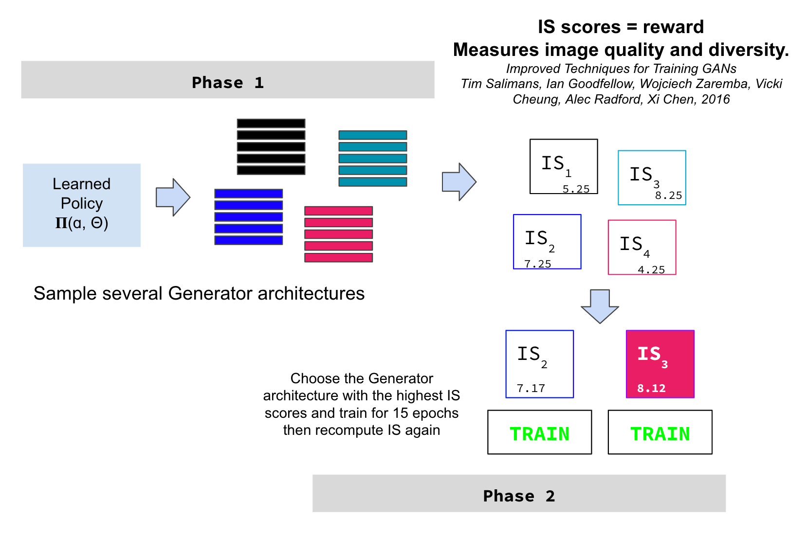
The training alternates between two phases. In Phase 1, the RNN controller parameters are fixed and several Generator architectures are sampled (offered up as candidates) via the learned REINFORCE policy. AutoGAN uses a hinge loss (e.g. SVM loss) to train the Generator and Discriminator. In Phase II, the GAN parameters are fixed and the Controller is updated by scoring each child network (the k best) based on their Inception Score (IS), a measure of quality and diversity for the images generated. Recall, this is similar but varies from NAS's use of validation accuracy.
The IS score (Salimans, et al.) is the RL policy reward. Scores that are closer to the number of predictable classes (CIFAR-10 has 10 classes) such as 8.12 versus 5.25 are "better". The lowest IS possible is 1.0 and the highest is the number of classes from the classification model (consider 1000 classes in the ILSVRC 2012 dataset). IS works by getting the generated images and predicting their classes using InceptionV3. IS is calculated as the exponent of the KL-divergency averaged across all classes, where KL = log(y|x) - log(P(y)), where the P(y) is the marginal probability, or p(y|x) for all predictions from InceptionV3. I found a great reference to better explain: https://machinelearningmastery.com/how-to-implement-the-inception-score-from-scratch-for-evaluating-generated-images/
Training Details
Wang et al. experiment on CIFAR-10 and STL-10. No augmentation was used. For CIFAR-10, they use 50,000 for training and 10,000 for test (32 x 32 resolution). For STL-10 they use 5,000 images for training and the 100,000 image non-labeled training set (resized 48 x 48 resolution).
- Learning rate for both Generator and Discriminator = 2e-4
- Hinge loss
- Adam optimizer
- Generator batch_size = 64, Discriminator batch_size = 128
- Controller trained using Adam optimizer, learning rate = 3e-4
- AutoGAN searched for 90 iterations, trained 15 epochs, Controller trained for 30 steps
- Generated architectures trained for 50,000 iterations
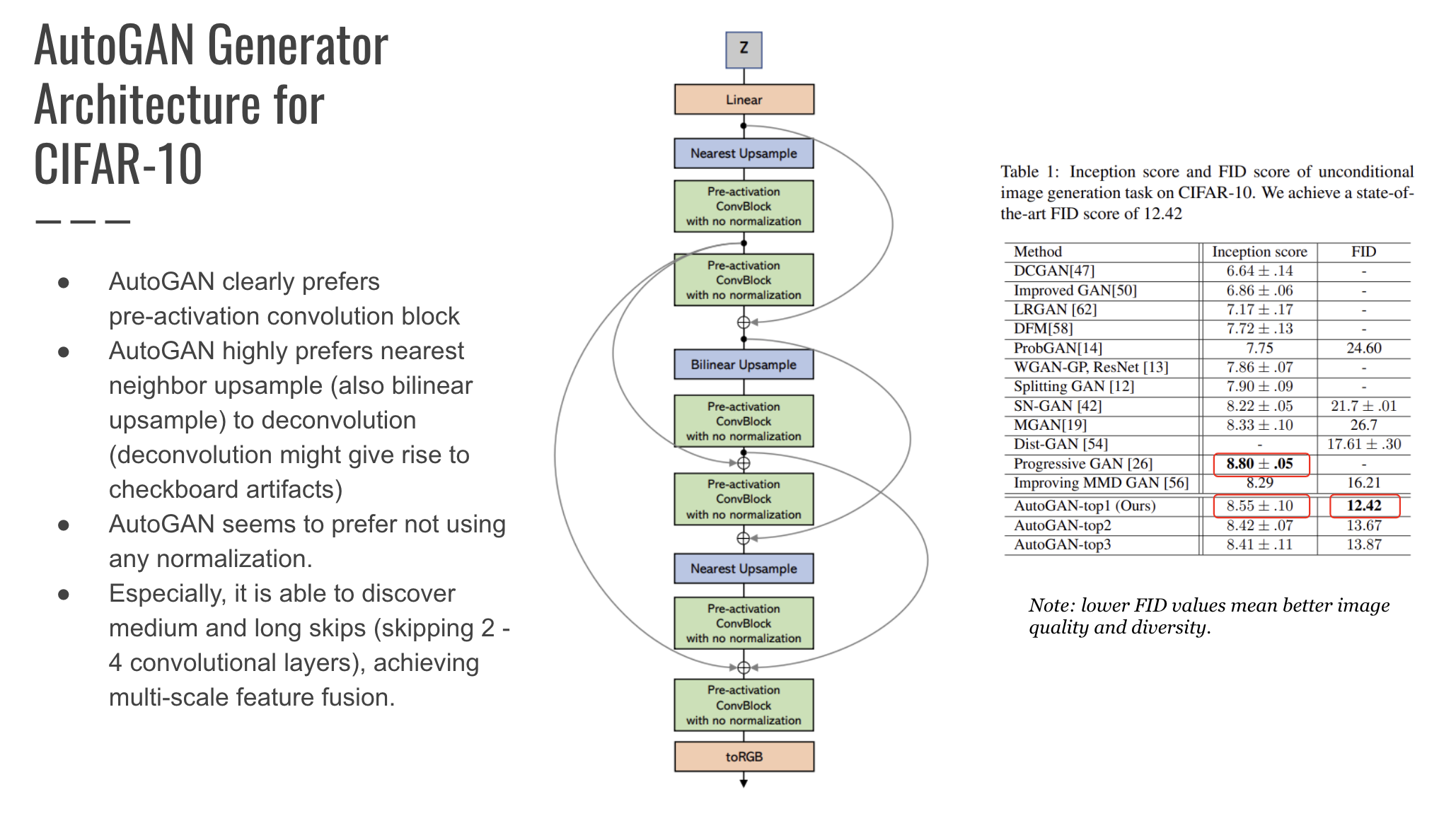
Below is the Generator architecture discovered by AutoGAN, bullets are directly from their paper denoting observations about this architecture - pre-activation convolutional blocks, skip connection discovery, and lack of normalization. On the CIFAR-10 image set, this discovered architecture (AutoGAN-Top1) obtained a FID score of 12.42 and IS of 8.55.
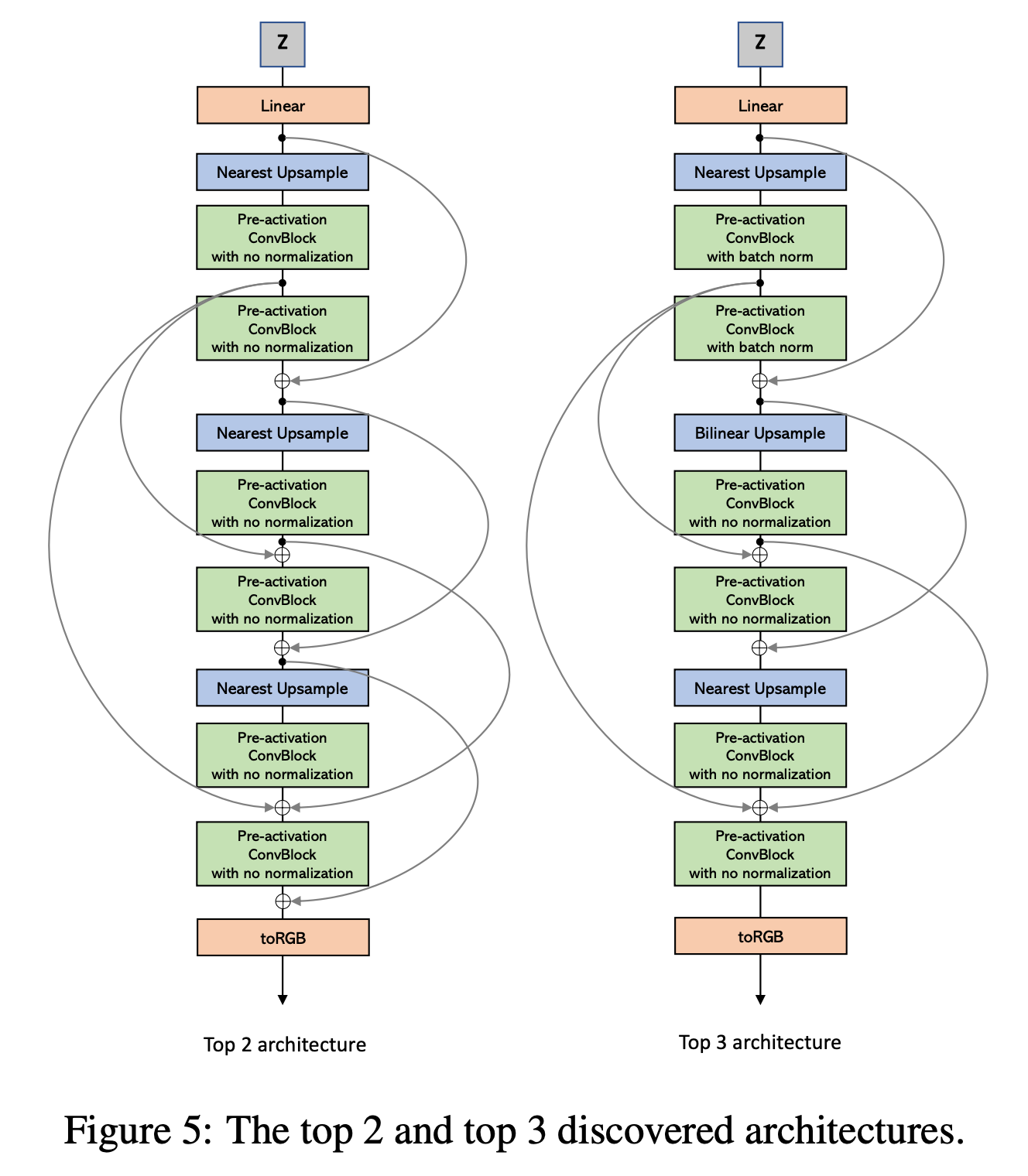
Below are the Top 2 and 3 discovered Generator architectures. Both blocks are similar, but the architectures differ in their number and locations of skip connections.
CIFAR-10 results:
STL-10 results:
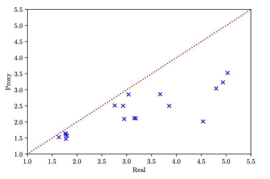
Going back to what Elksen et al. presented earlier on, Wang et al. makes good on the Performance Estimation Strategy part of NAS. Mainly, he trains candidate architectures in less time than a complete training session to find out if they're correlated and if the shorter-trained architecture is a good proxy and representative of a fully-trained model. Wang et al. plots the proxy IS versus the real IS scores and find a Spearman's rank correlation of 0.779, providing insight that the proxy training task is a fair estimation of the true IS value. They found that the proxy is actually conservative, underestimating the true IS since training was shorter than the real training task. This is valuable because candidate architectures can be quick trained to estimate future performance, before dedicating GPU resources for complete training. You may be wondering why they didn't calculate the FID instead of IS? The answer is that they decided to use IS as it was comparable to FID, but easier to calculate. Another strategy they use to train faster is "parameter dynamic-resetting", meaning that training stops if mode collapse occurs and there is a failure to converge, which they note at Section 3.2 occurs when they empirically observe the variance of the hinge loss to become very small. But they note that training without resetting takes 72 hours, but with resetting, it takes 43 hours.
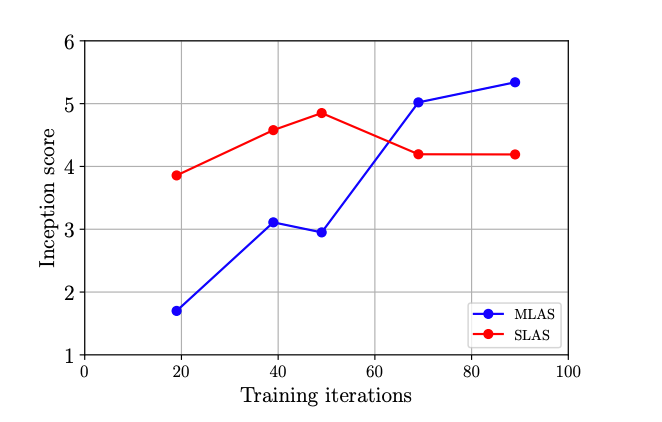
And finally, I had mentioned above how they use something called "multi-level architecture search" (MLAS) as the search strategy - uses multiple controllers to search for different combinations of blocks. They tested MLAS versus SLAS which sweeps the space to find a full CNN at once. SLAS starts off strong with a higher IS but MLAS catches up and beats the IS score. I'm not sure which AutoGAN this is for, since their top 3 yield IS scores above 8.41 +/-.11. They talk about how this decreases training time since SLAS is slow to train, but I suppose I'm not clear about why and how MLAS overtook SLAS in the IS which they didn't cover in the paper.
Well, that's it. There is a follow-up paper Learning Transferable Architectures for Scalable Image Recognition from the original 2016 Zoph & Le NAS paper I've reviewed, where Zoph et al., reduce the search space and also the training time from 800 GPUs for 28 days to 500 GPUs for 4 days. AmoebaNET uses an evolutionary algorithm instead of RL learning and uses the same search space as NASNet and uses TPUs but is still computational expensive. There are many more papers researching improvements to NAS, beyond only these.
I found a few YouTube interviews of one of the authors, Quoc Le of the NAS paper, in addition to other talks about NAS for your perusal.