Exploring Different Data Preprocessing Methods for LSTMs

I tend to focus a lot on how the data is wired, snipped, and prepared for models. I think the preprocessing steps of data lay the foundations by which all models are built and provides me a highly valuable exercise to understand the nooks and crannies of my dataset, especially when the data is new to me. I like focusing on the preprocessing step, also, as it teaches me about the quality of the data. And, that despite the sophistication of machine learning models: "Garbage in, Garbage out".
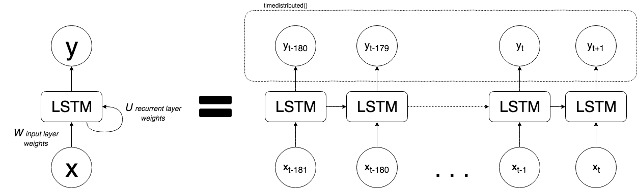
I've spent considerable time boiling the ocean to explore three specific methods for processing relational data for LSTMs. Each has some advantages and disadvantages. This blog post explores the first two methods. The third method which is using the keras timedistributed() wrapper consists of a very long n-length sequence of only one batch and is the method I demonstrated for the 2018 JupyterCon presentation. The Jupyter Notebook is here on my Github account here.
The Data
This dataset consists of 544 weekly observations of 6 different features for the area of Dallas, TX between 2007-04-28 and 2017-09-30.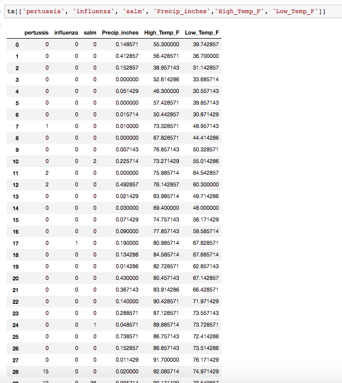
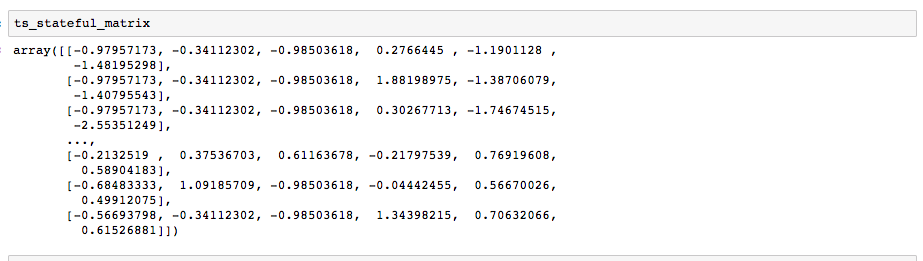
I normalized the data per below:
#for stateful LSTM, make pertussis the 1st feature in the column order
ts_stateful = ts[['pertussis', 'influenza', 'salm',
'Precip_inches','Low_Temp_F', 'High_Temp_F']]

#first convert to a 2d tensor of shape (timesteps, features)
ts_stateful_matrix = ts_stateful.values

#Normalize the whole matrix
mean = ts_stateful_matrix.mean(axis=0)
ts_stateful_matrix -= mean

std = ts_stateful_matrix.std(axis=0)
ts_stateful_matrix /= std
Method 1 - The "Bstriner" Method
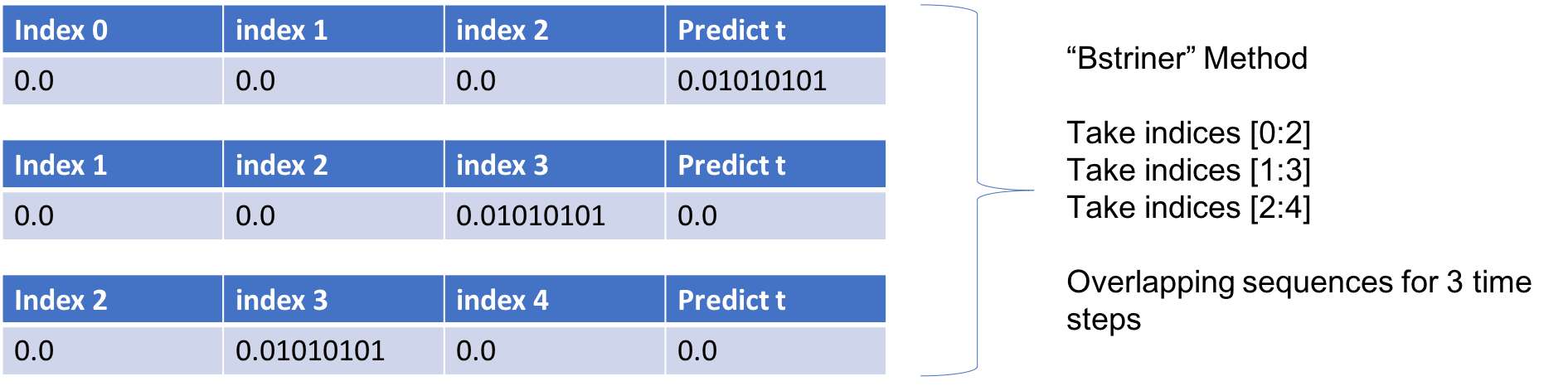
Upon exploring the Keras github forum (https://github.com/keras-team/keras/issues/4870), I came across a helpful post by someone named `bstriner`. In one answer, he writes on June 26, 2017: > Ideally you should break out overlapping windows. Instead of one sequence of 1870, you could have many sequences of let's say 20. Your sequences should be overlapping windows `[0-20], [1-21], [2-22]`, etc, so your final shape would be something like `(1850, 20, 14)`.Same process for your test data. Break into subsequences of the same length as training. You will have to play around with finding what a good subsequence length is. It is extremely important to have many different ways of slicing your data. If you train on just one super long sequence it will probably not learn anything interesting. Also, depending on what you decide to do, it may be better to generate subsequences as part of a generator function instead of doing it ahead of time. Check the keras docs for how to write a generator.Essentially if we want to look back 3 weeks for one variable, we want to create several samples of overlapping sequences like the below.
Method 2 - The Brownlee Method
This method comes from Jason Brownlee's blog "Machine Learning Mastery" where he has several discussions on time series. The below function has four arguments which you can find explained on the blog:My comments are in """ quotes documenting what the code he proposes is doing:
def series_to_supervised(data, n_in = 1, n_out = 1, dropnan=True):
  """says that if it's just a list of data, then there's one variable; otherwise if it's like mine, a n x m matrix, then the number of variables or features is the shape[1]. Eg: `(544, 6`) is shape so shape[1] in this case is == 6"""
    n_vars = 1 if type(data) is list else data.shape[1]
    df = pd.DataFrame(data)
    cols, names = list(), list() #empty lists
    # input sequence (t-n, ... t-1)
 """n_in is your lag that will be called in the get_sequence() function later on and is how many time steps you want your sequence to essentially "lag" or "look back". Eg. My data is in weeks. So I used a 3-week time window and set n_in = 3. The default for his function is 1. When you run the below code subbing in 3, it prints out 3 then 2 then 1. The function below is saying for i starting at 3 counting down to 1, append the column by shifting it out by 3, then 2, then 1. """
    for i in range (n_in, 0, -1):
       cols.append(df.shift(i))
 """This is creating a new column header 'var1(t-3)', 'var2(t-3)', 'var3(t-3)' ... 'var6(t-3)' and so on until your nth var. That's in my case, 6th var. It may not be clear now but this is the important quality of this function that allows the subsequent records generated to retain sequences. This is very similar to the "bstriner" method, in that it provides overlapping sequences, as we'll see later below."""
       names += [('var%d(t-%d)' % (j+1, i)) for j in range(n_vars)]
     # forecast sequence (t, t+1, ... t+n)
 """This is shifting out the next record in your sequence by the n_out timesteps. In my case I wanted to shift it out only 1 timestep which is the default setting, anyway. This results in the last column of the dataframe as 'var1(t)' where `var1` is my target of interest, and i'm only considering the next time step of one. If (the "else" statement) n_out was 2 timesteps, then we would end up getting an additional column `var1(t+1)`. If n_out ==3, then `var1(t)`, `var1(t+1)`, `var1(t+2)`. """
for i in range(0, n_out):
   cols.append(df.shift(-i))
       if i == 0:
            names += [('var%d(t)' % (j+1)) for j in range(n_vars)]
      else:
            names += [('var%d(t+%d)' % (j+1, i)) for j in range(n_vars)]
"""The rest is self-explanatory. The function concatenates all the columns created together into one dataframe and drops the NaN's"""
 # put it all together
     agg = concat(cols, axis=1)
     agg.columns = names
 # drop rows with NaN values
     if dropnan:
        agg.dropna(inplace=True)
     return agg
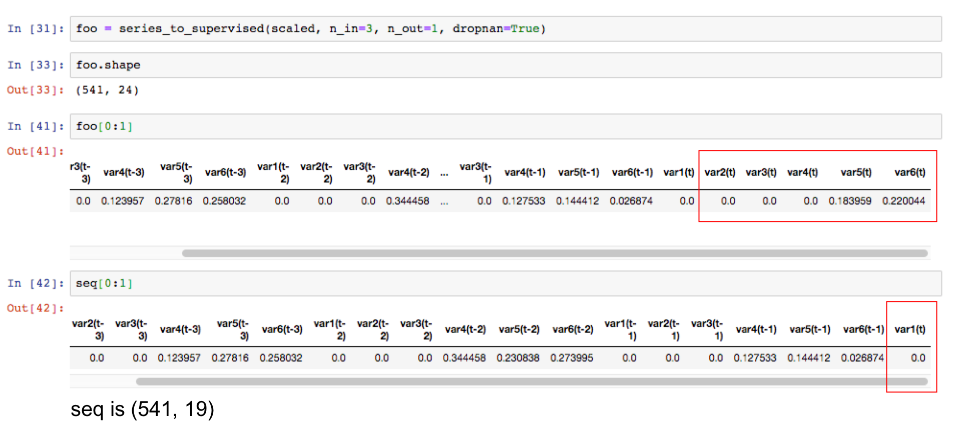
Now he moves on to generate the sequence maker. it's important to understand how the input variables in the sequence generator function:
def get_sequence(data, n_past, nth_var=1, n_forecast=1, dropnan=True) map to the function
def series_to_supervised(data, n_in = 1, n_out = 1, dropnan=True), like so:
An additional input into def get_sequence() is nth_var which is handy for the user to define which variable in the data is the target of interest. For me, it was the first variable in my 6-dimensional feature set.
def get_sequence(data, n_past, nth_var=1, n_forecast=1, dropnan=True):
    seq = series_to_supervised(data, n_past, n_forecast, dropnan)
    # drop columns we don't want to predict
"""This is a clean up process, essentially. It drops the current timestep for var2, var3, var4, var5, and var6, keeping only var1 which is my target I want to forecast."""
    col_index = range(seq.shape[1]-data.shape[1],seq.shape[1])
    del col_index[nth_var-1]
    seq.drop(seq.columns[col_index], axis=1, inplace=True)
    return seq
Understanding the Sequence Results
It's important to understand that the sequence generated preserves the patterns in the time series. This is the output csv of the sequence just generated for 6 variables with 3 timesteps of lookback and 1 time step of look forward specifically for just one variable, var1(t).
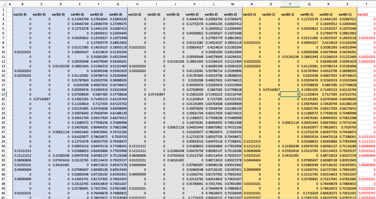
You'll notice that the target variable is included in the sequence. While in supervised machine learning use cases, you'd consider this as "target leakage" in this case, we need it as a part of our weekly sequence. The model learns on the past trends of all the variables including our target.
What I've done here is hide the other variables 2 through 6, so that you could see how the sequences overlap to capture three timesteps of lookback.
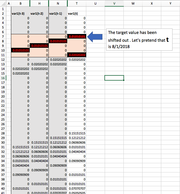
Explaining it here like so. Let's pretend today is August 29, 2018 and that four weeks ago it was the week of August 1st. You can see that on 8/1, t this week was a 0.01010101. The next week on 8/7, you'll see that 8/1 then became the week prior and the sequence reflects that at t-1, and so on. By the time we get to 8/29, t-3 is no longer in our current sequence. This week, 8/29's, value is now t == 0.02020202.
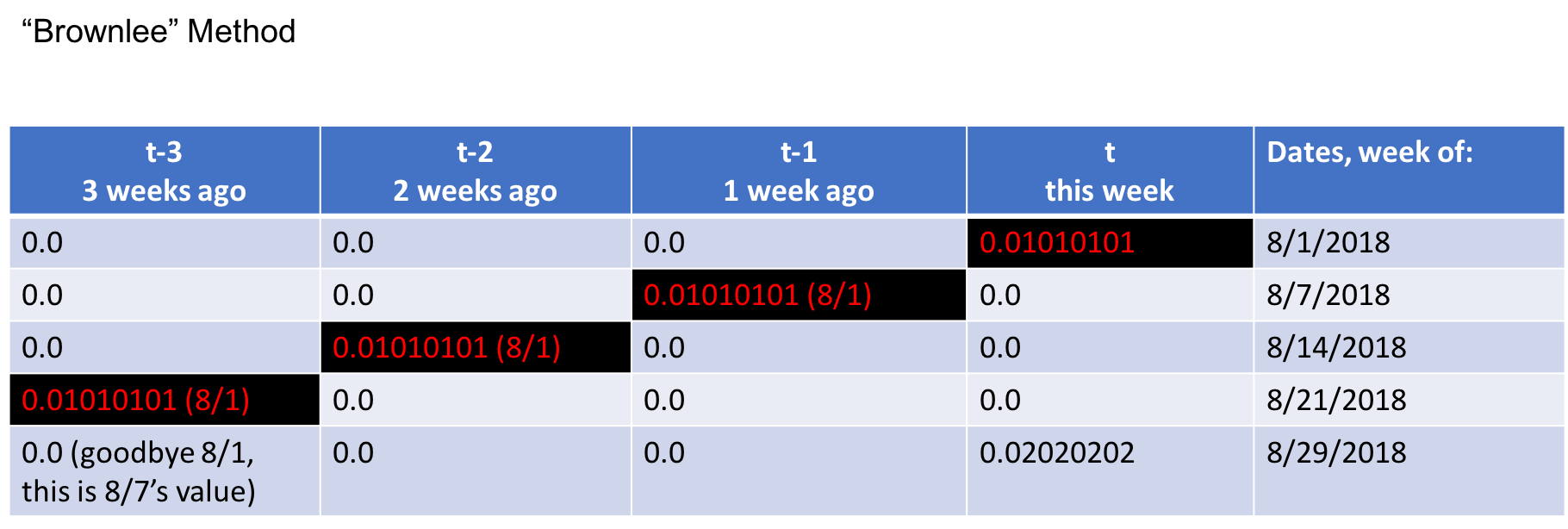
You can see how this is similar to the "BStriner" Method proposed above:

Method 3
Knowing that LSTMs are suitable for sequences with long-term chronological patterns in their series, I explored the idea of generating one long single batch of 181 timesteps for each of the 5 variables (1, 181, 5) for my training set, 181 timesteps (1, 181, 5) for my validation set, and 181 timesteps (1, 181, 5) for my test set (181 * 3 = 543, since I shifted the pertussis forecast out by one timestep, I lost one week of forecast fro 544 to 543).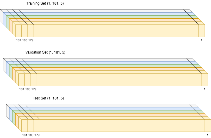
I implemented this method in the Jupyter Notebook is here on my Github account here.
Method 4 - The Chollet Generator Method
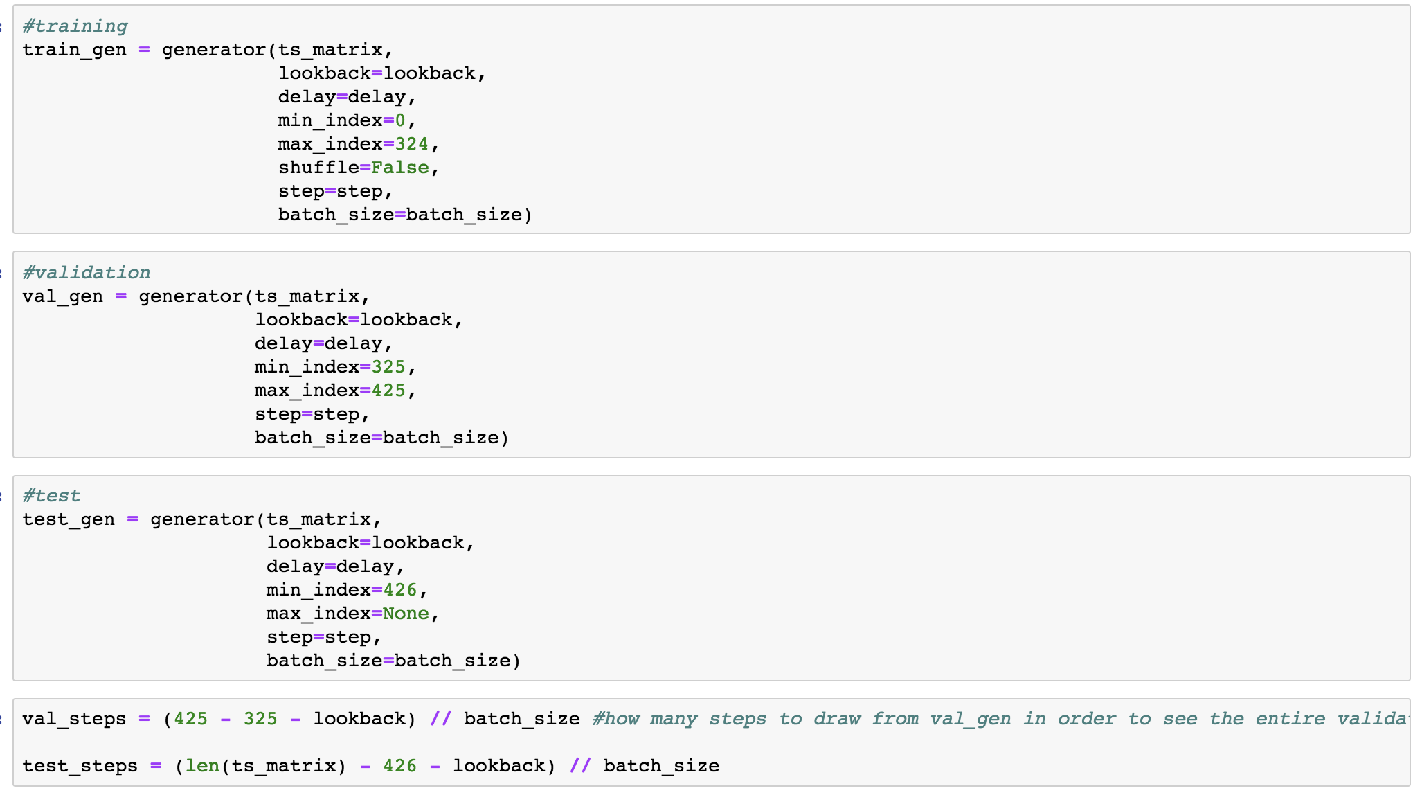
This method comes from Chollet's book "Deep Learning with Python" in Chapter 6 "Deep learning for text and sequences" on Page 207, "Advanced use of recurrent neural networks" Listing 6.33 on Page 211. Using this method is an automated way of generating the sequences and look back window described in the "brstiner" method. Let's explore the performance of this method in the next, upcoming blog post.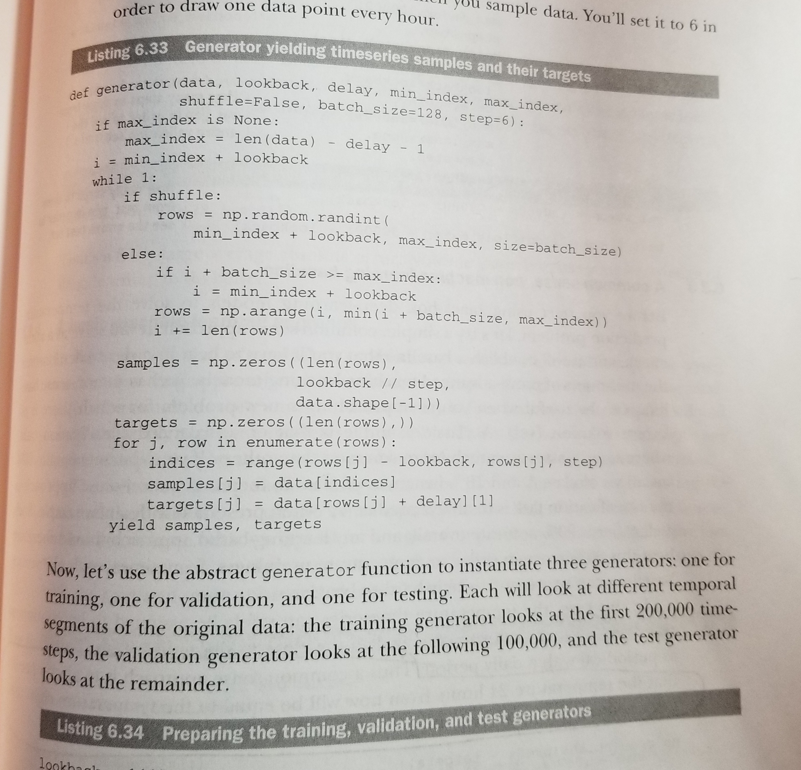
lookback = 32
step = 4
delay = 1
batch_size = 32

def generator(data, lookback, delay, min_index, max_index,
          shuffle=False, batch_size=batch_size, step=step):
   if max_index is None:
       max_index = len(data) - delay - 1
   i = min_index + lookback
   while 1:
       if shuffle:
          rows = np.random.randint(
            min_index + lookback, max_index, size=batch_size)
      else:
         if i + batch_size >= max_index:
            i = min_index + lookback
         rows = np.arange(i, min(i + batch_size, max_index))
         i += len(rows)

     samples = np.zeros((len(rows),
                       lookback // step,
                       data.shape[-1]))
     targets = np.zeros((len(rows),))
     for j, row in enumerate(rows):
        indices = range(rows[j] - lookback, rows[j], step)
        samples[j] = data[indices]
  """Note the [1] which indicates that the target is the second variable in this feature set. We need to change this to [0] since its our first."""
        targets[j] = data[rows[j] + delay][1]
     yield samples, targets
We then fit the generators:
from keras.models import Sequential
from keras import layers
from keras.optimizers import RMSprop

#model.fit_generator means Fits the model on data yielded batch-by-batch by a Python generator.

model = Sequential()

model.add(layers.Flatten(input_shape=(lookback // step,
ts_matrix.shape[-1])))

model.add(layers.Dense(1))

model.compile(optimizer=RMSprop(), loss='mae')

history = model.fit_generator(train_gen,
                          steps_per_epoch=30,
                          epochs=30,
                          validation_data=val_gen,
                          validation_steps=val_steps)