Murder Accountability Project - Part 3 Predicting Murder by a Voting Classifier

Introduction

On Twitter I found an excellent Github repo with several hands on Python notebooks as tutorials. Particularly this one notebook by Aurelien Geron, author of Machine Learning and Deep Learning in python using Scikit-Learn and TensorFlow, has a well documented tutorial on Voting Classifiers, Gradient Boosting, and Random Forest Classifiers (Bagging), all the types callable under the sklearn.ensemble API. One of the most awesome books I've seen in a while:

Notable tangent

While perusing the repo, I also checked out Notebook #2. Check out the below snippet of his code to get schooled on writing kick-ass pipelines.

For example, straight out of his notebook:

num_attribs = list(housing_num)
cat_attribs = ["ocean_proximity"]

This pipeline selects numerical dtypes from the dataframe, imputes missing values using the median, and uses a standard scaler normalizing values

num_pipeline = Pipeline([
    ('selector', DataFrameSelector(num_attribs)),
    ('imputer', Imputer(strategy="median")),
    ('attribs_adder', CombinedAttributesAdder()),
    ('std_scaler', StandardScaler()),
])

Then this pipeline selects categorical dtypes from the dataframe, uses the label binarizer to essentially factorize them

cat_pipeline = Pipeline([
    ('selector', DataFrameSelector(cat_attribs)),
    ('label_binarizer', LabelBinarizer()),
])

from sklearn.pipeline import FeatureUnion

This is the full pipeline telling the pipeline to first normalize numeric data, then categorical data

full_pipeline = FeatureUnion(transformer_list=[
    ("num_pipeline", num_pipeline),
    ("cat_pipeline", cat_pipeline),
])

Now he runs it and the housing dataset is cleaned.

housing_prepared = full_pipeline.fit_transform(housing)

The final pipeline he makes prepares the data like above, conducts feature selection by selecting say k=5 of the top features he wants which is more time-saving then doing a RandomForestClassifier feature_importance function, and then he finally makes the prediction using an SVR algorithm.

prepare_select_and_predict_pipeline = Pipeline([
  ('preparation', full_pipeline),
  ('feature_selection', 
  TopFeatureSelector(feature_importances, k)),
    ('svm_reg', SVR(**rnd_search.best_params_))
])

prepare_select_and_predict_pipeline.fit(housing, 
housing_labels)

I went on a tangent there to discuss pipelines, because you can automate the ML process so much by making clever ones. For example, use PCA to reduce a high-dimensional dataframe, one-hot-encode, and then run a logistic regression. Or, use it to vectorize text, run TF-IDF and then apply a Naive Bayes text classifier. The combinations are endless, and from industry experience, I can assert that pipelines are make/break for a production-grade machine learning application.

For those of you who want to explore his notebook, I'd also recommend reviewing his results of using sklearn.model_selection.GridSearchCV compared to sklearn.model_selection.RandomizedSearchCV. Randomized Search runs faster than Grid Search because,

"In contrast to GridSearchCV, not all parameter values are tried out, but rather a fixed number of parameter settings is sampled from the specified distributions."

Stacked Ensembling
Also something else I learned which I'll try to do in my next post, is to try out the h2o package as an exercise in writing a stacked ensemble, where the model will learn the weights, as opposed to manually entering them like I'm doing in this post.

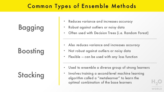
As I'm still learning about how to create a stacked ensemble, I'm providing some courtesy-of-h2o slides here:

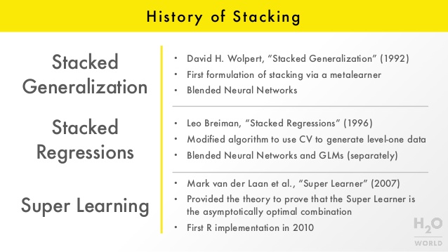
And the history of ensembling:

This is also my excuse to post a photo of Katy Perry "voting" - she's our data science Dark Horse!

Soft Voting Classifier

This is a binary classification problem to predict 0 = Manslaughter by Negligence or 1 = Murder or Manslaughter.

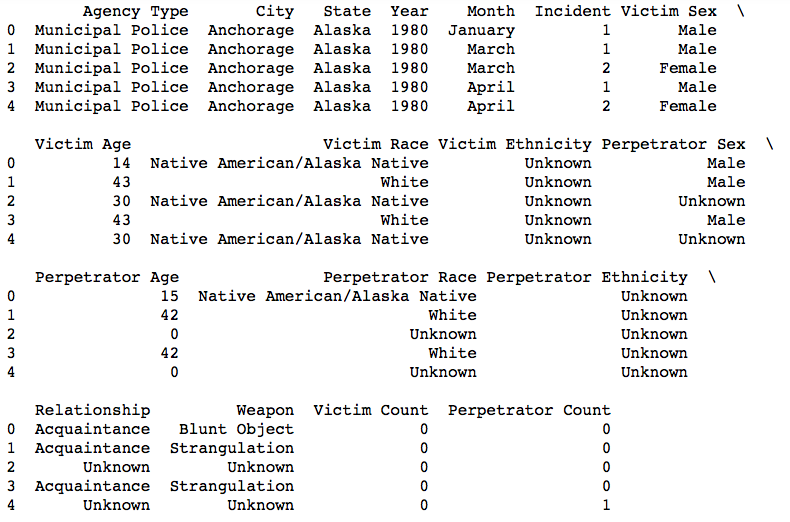
df = data2.copy()
df.dtypes

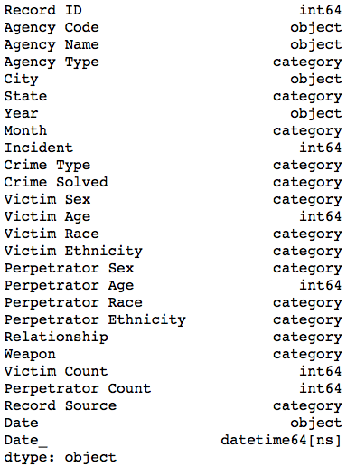
#convert year to int
df['Year'] = df['Year'].astype(int)
#just get the features and the target first 
X_df = (df.drop(['Record ID', 'Agency Code', 'Agency Name', 'Date_', 'Date', 'Crime Type', 'Crime Solved','Record Source'], axis=1))
y_df = df['Crime Type']

X_df.head()

y_df.head()

X_df["City"] = X_df["City"].astype('category')

#get dummies to OHE
X = pd.get_dummies(X_df, columns=["Agency Type", "City", "State", "Month", "Victim Sex", "Victim Race", "Victim Ethnicity", "Perpetrator Sex", "Perpetrator Race", "Perpetrator Ethnicity", "Relationship", "Weapon"])
X.shape #(638454, 1924)

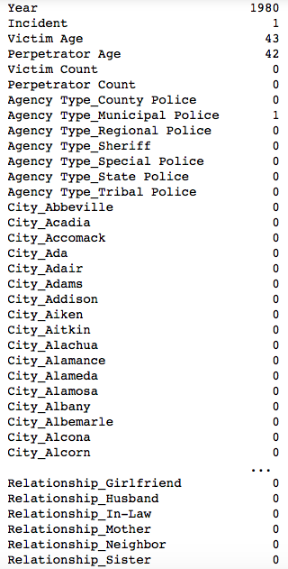
#look at the first index 
X.iloc[1]

#encode the target
le = preprocessing.LabelEncoder()
Y = le.fit(y_df)
Y.classes_
#'manslaughter by negligence' is 0, and 'murder or manslaughter' is 1

#now put it into an array
Y = le.transform(y_df)
#convert X into an array 
X_fin = X.values

At this point, we have a very high dimensional set of features at 1,924 features. We need to reduce this. Let's use select best features as preprocessing, dimensionality reduction, prior to the estimation.

from sklearn.ensemble import ExtraTreesClassifier
from sklearn.feature_selection import SelectFromModel

clf = ExtraTreesClassifier()
clf = clf.fit(X_fin, Y)
clf.feature_importances_  
model = SelectFromModel(clf, prefit=True)
X_new = model.transform(X)

#new number of features - reduced from 1924 to 203 features 
X_new.shape #(638454, 203)

Using X_new as the new data.

X_train, X_test, y_train, y_test = sklearn.cross_validation.train_test_split(X_new, Y, test_size=0.30, random_state=0)
print(X_train.shape)
print(X_test.shape)
print(y_train.shape)
print(y_test.shape)

Set up the voting classifier

The weights of 1, 5, 1, means that the probabilities from the RandomForestClassifier will be weighted at 5 times greater than the LogisticRegression and GaussianNB classifiers. You can adjust this manually. Hence, if this is not the optimal combination, using a meta-learner per h2o may be a better route. Also, you'll notice I didn't run a GridsearchCV on the classifiers. In my follow-up post, I'll build a pipeline to do this.

from sklearn.linear_model import LogisticRegression
from sklearn.naive_bayes import GaussianNB
from sklearn.ensemble import RandomForestClassifier
from sklearn.ensemble import VotingClassifier

clf1 = LogisticRegression(random_state=123)
clf2 = RandomForestClassifier(random_state=123)
clf3 = GaussianNB()

eclf = VotingClassifier(estimators=[('lr', clf1), ('rf', clf2), ('gnb', clf3)],voting='soft', weights=[1, 5, 1])

Predict class probabilities for all classifiers:

probas = [c.fit(X_train, y_train).predict_proba(X_test) for c in (clf1, clf2, clf3, eclf)]

Get the class probabilities for the first sample in the dataset:

class1_1 = [pr[0, 0] for pr in probas]
class2_1 = [pr[0, 1] for pr in probas]

print(probas)

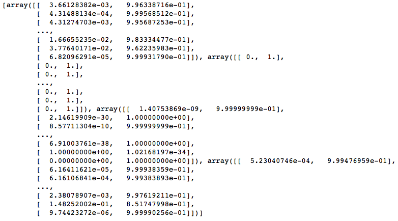
This tells me that for the first record in X_test, the probabilities for class 1 which is Manslaughter by Negligence:

0.3% for clf1, 0% for clf2, .0000001% for clf3, and .05% for eclf

class1_1

This tells me that for the first record in X_test, the probabilities for class 2 which is Murder or Manslaughter:

99.633% clf1, 100% clf2, 99.999% clf3, 99.947% for eclf

class2_1

Plot class probabilities using this tutorial from sklearn: http://scikit-learn.org/stable/auto_examples/ensemble/plot_voting_probas.html

N = 4  # number of groups:  the 3 clf's and the ensemble
ind = np.arange(N)  # group positions
width = 0.35  # bar width

fig, ax = plt.subplots()

# bars for classifier 1-3
p1 = ax.bar(ind, np.hstack(([class1_1[:-1], [0]])), 
    width, color='red', edgecolor='k')
p2 = ax.bar(ind + width, np.hstack(([class2_1[:-1], [0]])), width, color='green', edgecolor='k')

# bars for VotingClassifier
p3 = ax.bar(ind, [0, 0, 0, class1_1[-1]], width,
        color='blue', edgecolor='k')
p4 = ax.bar(ind + width, [0, 0, 0, class2_1[-1]], width,
        color='steelblue', edgecolor='k')

# plot annotations
plt.axvline(2.8, color='k', linestyle='dashed')
ax.set_xticks(ind + width)
ax.set_xticklabels(['LogisticRegression\nweight 1',
                'GaussianNB\nweight 1',
                'RandomForestClassifier\nweight 5',
                'VotingClassifier\n(averageprobabilities)'],
               rotation=40, 
               ha='right')
plt.ylim([0, 1])
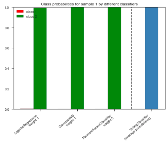
plt.title('Class probabilities for sample 1 by different classifiers')
plt.legend([p1[0], p2[0]], ['class 1', 'class 2'], loc='upper left')
plt.show()

Run 5-fold cross validation

from sklearn import model_selection
seed=7
kfold = model_selection.KFold(n_splits=5, random_state=seed)
results = model_selection.cross_val_score(eclf, X_train, y_train, cv=kfold)
print(results.mean())

0.986664190242

Important Considerations

1. Utility of this model in practice. It's hardly useful to write a model where the user needs to enter 203 features in order to make a prediction. Now that I've gone through the exercise of making this voting classifier, it'll be important to start at the top again and take these into account:

2. Target Leakage. What features are available at the time of prediction? If a police officer or investigator were going to use this, it's most likely she will have a limited amount of features like the weapon, relationship, time, date, city, state, victim demographics.

3. Feature Importance. With the features in-mind that are not going to leak, then before one-hot-encoding, run feature selection to identify the most important.

4. Class imbalance. There is very little red regarding class 1 which is 'Manslaughter by Negligence' because all the classifiers predicted close to 0% probability of of the test case being this category, and most predicted 'Murder or Manslaughter'. Now you might be wondering about imbalance of the target set. The ratio of imbalance is 69 cases of class 0 (or Murder) to every one case of class 1 (or Negligence).

Looking at Class Imbalance
As a result, a problem that we may have here is to deal with class imbalance.

from sklearn.preprocessing import LabelEncoder

lb_make = LabelEncoder()
target_types = pd.DataFrame(lb_make.fit_transform(y_df))

target_types.hist()

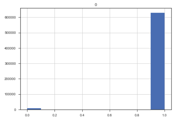
#Ratio of imbalance
len(target_types.loc[target_types[0] == 1]) / 
len(target_types.loc[target_types[0] == 0])