Murder Accountability Project - Part 1 Data Prep and Map

The first job I ever had out of college was as an autopsy tech assistant at the Fulton County Medical Examiner's Office. I helped out first as an intern at DeKalb County on death scene investigations, and later after college in Fulton County helping the techs perform autopsies and conduct organ procurement. That was one of the best professional experiences of my life providing me the opportunity understand the relationship between law enforcement and medicine, specifically forensic pathology. So, this dataset really was interesting to me, and while the below is a pretty basic data science post, I'll continue to work on this throughout the year to see if I can generate some new insights.

The Data
This data is from Kaggle, available here: https://www.kaggle.com/murderaccountability/homicide-reports. A little overview about it:
The Murder Accountability Project is the most complete database of homicides in the United States currently available. This dataset includes murders from the FBI's Supplementary Homicide Report from 1976 to the present and Freedom of Information Act data on more than 22,000 homicides that were not reported to the Justice Department. This dataset includes the age, race, sex, ethnicity of victims and perpetrators, in addition to the relationship between the victim and perpetrator and weapon used.
Part 1 - Data Prep
data = pd.read_csv(".../database.csv")
print("There are", len(data), "records.")
This dataset has 638,454 records, consisting of 18 object variables and 6 integer variables a total of 24 variables.
print(data.dtypes.value_counts())
print(data.dtypes)
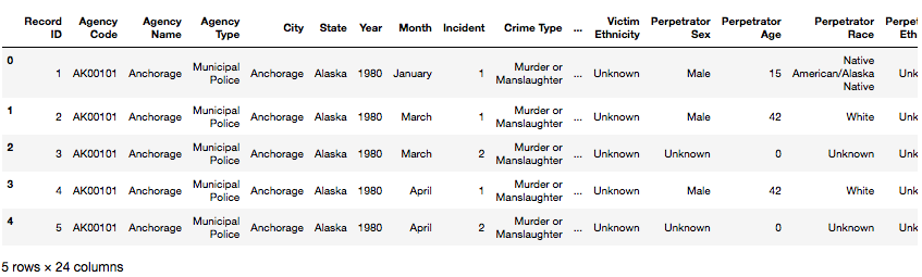
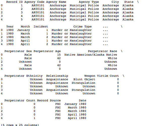
print(data.head())
How many unique variables for each of those 18 object variables? Let's get the unique category names of each object variable, using the .nunique() command
print("Number unique Agency Name vars", data['Agency Name'].nunique())
Number unique Agency Name vars 9216
Number unique Agency Code vars 12003
Number unique Agency Type vars 7
Number unique City 1782
Number unique State 51
Number unique Month 12
Number unique Crime Type 2
Number unique Crime Solved 2
Number unique Victim Sex 3
Number unique Victim Ethnicity 3
Number unique Perpetrator Sex 3
Number unique Perpetrator Age 191
Number unique Perpetrator Race 5
Number unique Relationship 28
Number unique Weapon 16
Number unique Record Source 2
Let's look at Record ID 3. Here, Record ID 3 was a 30 yo female victim Native American/Alaska Native killed in March 1980 whose Perpetrator demographics are completed unknown
print(data.loc[2])
In a different case, Record ID == 5000, this is a 21 yo White Male victim of Murder or Manslaughter in Fairfield, CT. Killed in October 1980 by a 26 yo White Male, a stranger, who used a handgun
print(data.loc[4999])
Change Year to datetime. Convert to categorical: 'Agency Type', 'State', 'Month', 'Crime Type', 'Crime Solved', 'Victim Sex', 'Victim Race', 'Victim Ethnicity', 'Perpetrator Sex', 'Perpetrator Race', 'Perpetrator Ethnicity', 'Relationship', 'Weapon', 'Record Source', and Convert 'Perpetrator Age' to integer.
data2 = data.copy()
data2['Year'] = data2['Year'].astype(str)
data2['Month'] = data2['Month'].astype(str)
print(data2['Year'].unique())
print(data2['Month'].unique())
data2['Date'] = data2['Month'] + " "+ data2['Year']
Convert the date into a single month-year
data2['Date'] = data2['Month'] + " " + data2['Year']
data2['Date_'] =  pd.to_datetime(data2['Date'], format='%B %Y')
print(data2.dtypes)
Make sure it converted to only year datetimes
data2['Date_'].loc[:10]
Convert variables into categories
def ascategory(cols, df):
for col in cols:
	df[col] = df[col].astype('category')
  all_cols = ['Agency Type',
        'State',
        'Month',
        'Crime Type',
        'Crime Solved',
        'Victim Sex', 'Victim Race',
        'Victim Ethnicity',
        'Perpetrator Sex',
        'Perpetrator Race',
        'Perpetrator Ethnicity',
        'Relationship',
        'Weapon',
        'Record Source'
   ]

ascategory(all_cols, data2)
print(data2.dtypes)
data2['Perpetrator Age'] = data2['Perpetrator Age'].astype(str)
data2['Perpetrator Age'] = data2['Perpetrator Age'].str.replace(' ', '0')
data2['Perpetrator Age'].unique()
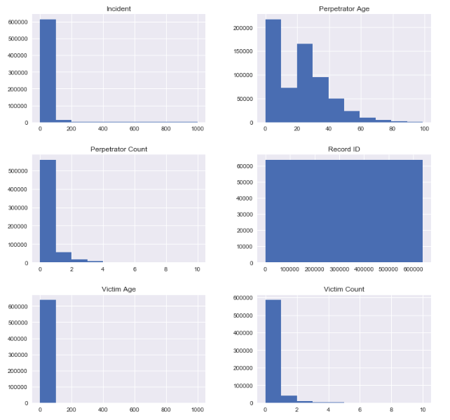
Histogram of all integer dtypes - Record ID isn't relevant.
(data2.select_dtypes(include=['int64'])).hist(figsize=(12,12))
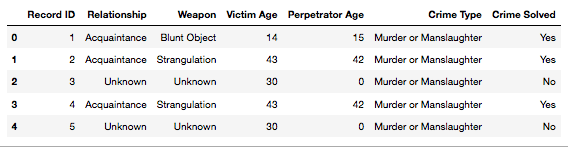
s1 = data2[['Record ID', 'Relationship', 'Weapon', 'Victim Age', 'Perpetrator Age', 'Crime Type', 'Crime Solved']].copy()
s1.head()
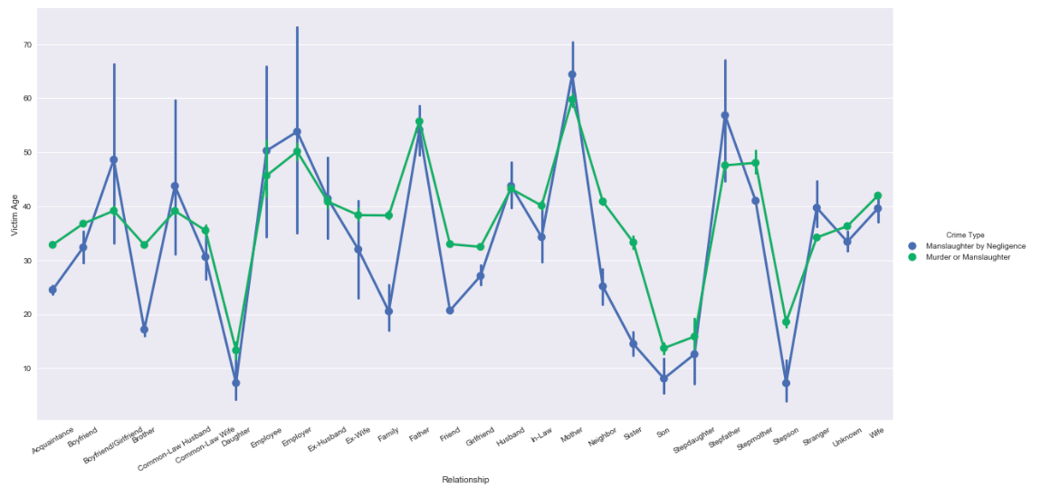
g = sns.factorplot(x='Relationship', y='Victim Age', hue='Crime Type', data=s1, kind="point", size=8, aspect=2)

g.set_xticklabels(rotation=30)
Shows that older people are the victims of murder by family (in-law, mother, family), whereas children are victims or murder by family as well (Boyfriend/Girlfriend, Common-law Wife, Son, Stepdaughter, Stepson).
Part 2 - Mapping Murders in States
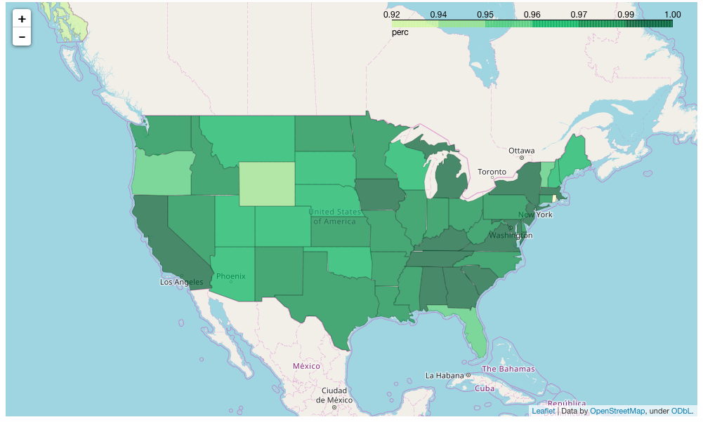
Display on a map, the percentage of each Crime Type out of All Crimes for each state. Build one using the Python package folium.
import folium
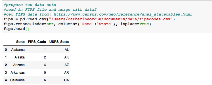
Prepare two data sets and read in FIPS file and merge with data2. Get the FIPS data from: https://www.census.gov/geo/reference/ansi_statetables.html
fips = pd.read_csv("/Users/catherineordun/Documents/data/fipscodes.csv")
fips.rename(index=str, columns={'Name':'State'}, inplace=True)
fips.head()
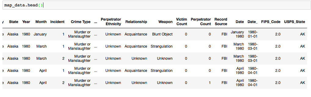
Now, merge with data2 to get the state abbreviations
map_data = pd.merge(data2, fips, on="State", how='left')
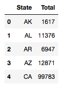
Get the total records for each state.
map_counts = pd.pivot_table(map_data,index=["USPS_State"],values=["Record ID"],aggfunc=[len])
#reshape
mc1 = map_counts.reset_index()
mc1.columns.droplevel()
mc1.columns = ['State', 'Total']
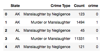
mc2 = map_crime.reset_index()
mc2.columns = mc2.columns.droplevel()
mc2.columns = ['State', 'Crime Type', 'Count']
mc2['crime'] = pd.factorize(mc2['Crime Type'])[0]
mc2.head()
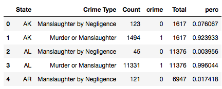
crimecount = pd.merge(mc2, mc1, on='State')
crimecount['perc'] = crimecount['Count'] /
crimecount['Total']
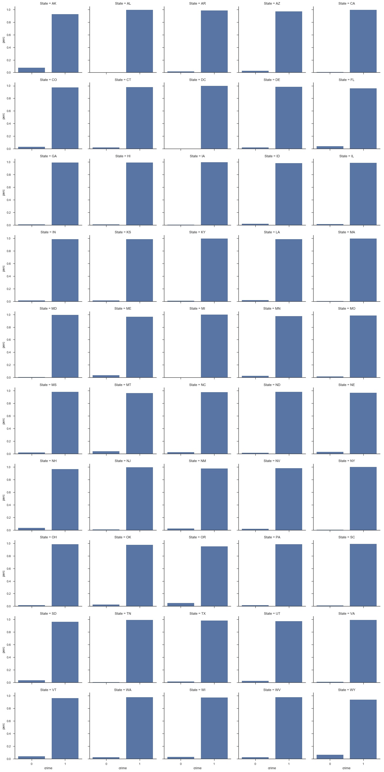
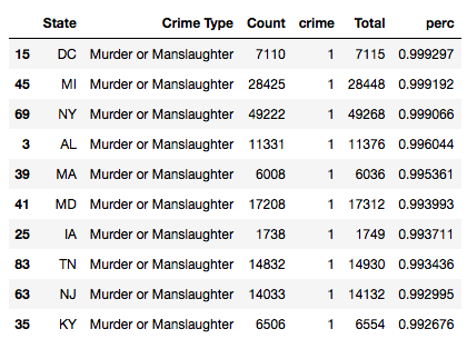
How does'Murder or Manslaughter', compare to 'Manslaughter by Negligence', for each state based on the total percentage of all records during this time frame?
sns.set(style="ticks")
g = sns.FacetGrid(crimecount, col="State", col_wrap=5, size=3.5)
g = g.map(sns.barplot, "crime", "perc")
You need to download the us-states.json file from here: https://github.com/python-visualization/folium/tree/master/examples/data
state_geo = r'/Users/catherineordun/Documents/data/us-states.json' ((crimecount.loc[(crimecount['crime']==1)]).sort_values(by ='perc', ascending=False)).head(10)
Let Folium determine the scale
map_2 = folium.Map(location=[48, -102], zoom_start=3)
map_2.choropleth(geo_path=state_geo, data=(crimecount.loc[(crimecount['crime']==1)]),
         columns=['State', 'perc'],
         key_on='feature.id',
         fill_color='YlGn', fill_opacity=0.7, line_opacity=0.2,
         legend_name='perc')
States by percentage of total as being murders
display(map_2)