Predicting Animal Shelter Outcomes

I was preparing to give a talk for some important Veteran Advocacy Non-Profits here in DC the other day, and wanted to provide an easy to understand example of machine learning and classification. So, I found this interesting data set on Kaggle from the Austin Animal Center. This subject is near to my heart, since my dog, Stella was a rescue from the Lost Dog Foundation here in Northern Virginia.
So, let's get started with building a model to predict categories out animal shelter outcomes. First, the data looks like this:
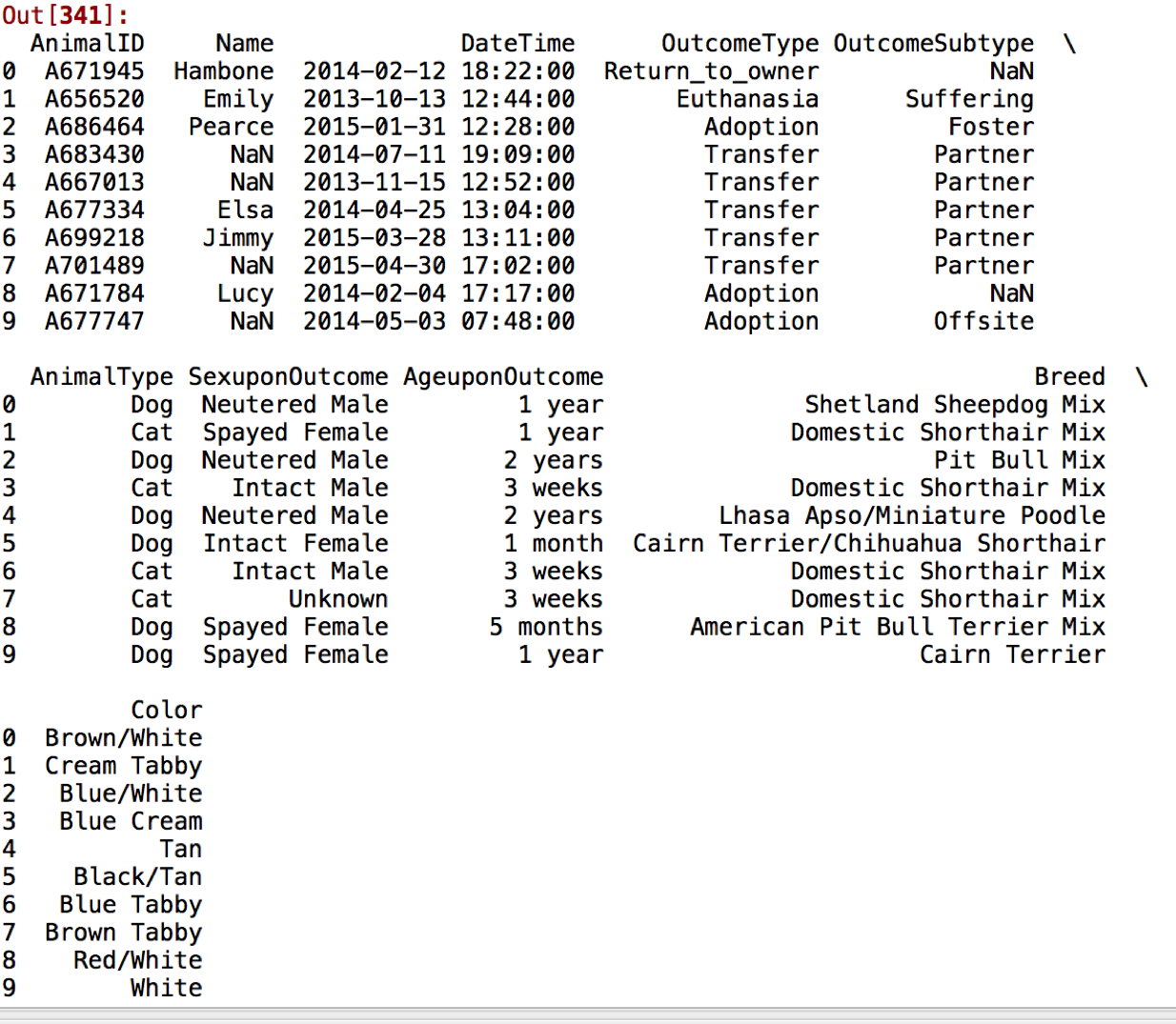
Pretty standard categorical variables like OutcomeType, Color, Breed, as well as features that we'll have to convert into integers like AgeuponOutcome. Based on this dataset, there are two big questions I'd like to ask of the data:
Yup, you guessed it: Data Cleaning
This dataset required some basic clean-up. I didn't focus attention on the test set this time, because the test set itself didn't contain the Outcome Variable that I wanted to predict. What I did instead for the purpose of this exercise, was split up the training set into a 70/30 split.
train = pd.read_csv("/Users/catherineordun/Documents/scripts/data/animal_train.csv")
test = pd.read_csv("/Users/catherineordun/Documents/scripts/data/animal_test.csv")

#convert to datetime
train['Date'] = pd.to_datetime(train['DateTime'])
test['Date'] =  pd.to_datetime(test['DateTime'])

#Convert variables into categories
def ascategory(cols, df):
for col in cols:
	df[col] = df[col].astype('category')
 all_cols = ['OutcomeType',
        'OutcomeSubtype',
        'AnimalType',
        'SexuponOutcome',
        'Breed',
        'Color']
#test does not have Outcomes
all_cols2 = ['AnimalType',
        'SexuponOutcome',
        'Breed',
        'Color']
ascategory(all_cols, train)
ascategory(all_cols2, test)
Test data types:
ID int64
Name object
DateTime object
AnimalType object
SexuponOutcome object
AgeuponOutcome object
Breed object
Color object
Date datetime64[ns]
#convert AgeuponOutcome to integer
train['AgeuponOutcome'] =
train['AgeuponOutcome'].astype(str)
train['AgeuponOutcome'].fillna(value=0)
Standardize all ages in terms of months:
*note I was having some markup problems here, so if you copy this code, ensure there is no '_' space between 'loc' and the bracket [. Remember walk through the code yourself so you understand it!
train.loc [(train['AgeuponOutcome'].str.contains('year')), 'Age_Mos'] = (train['AgeuponOutcome'].str.extract('(\d+)').astype(float))*12

train.loc [(train['AgeuponOutcome'].str.contains('week')), 'Age_Mos'] = (train['AgeuponOutcome'].str.extract('(\d+)').astype(float))/4

train.loc [(train['AgeuponOutcome'].str.contains('month')), 'Age_Mos'] = (train['AgeuponOutcome'].str.extract('(\d+)').astype(float))

train.loc [(train['AgeuponOutcome'].str.contains('day')), 'Age_Mos'] = (train['AgeuponOutcome'].str.extract('(\d+)').astype(float))/30

#factorize
train['outcome'] = pd.factorize(train['OutcomeType'])[0]

train['subtype'] = pd.factorize(train['OutcomeSubtype'])[0]

train['animal'] = pd.factorize(train['AnimalType'])[0]

train['sex'] = pd.factorize(train['SexuponOutcome'])[0]

train['breed'] = pd.factorize(train['Breed'])[0]

train['color'] = pd.factorize(train['Color'])[0]

#NaN's were making the factored value -1, so I
replaced it with 16
train['subtype'].replace(-1, 16, inplace=True)
At this point I was also curious about whether the name of the animal made a difference? So, to test this idea, I just extracted the first character of the name.
 #Extract the first letter of the names - does that make a difference?
train['name_letter'] = (train['Name'].str.lower()).str[0]
train['name_'] = pd.factorize(train['name_letter'])[0]
train['name_'].replace(-1, 32, inplace=True)
Trends in Shelter Activity
#========MODEL
train_fin = train[['Date', 'Age_Mos', 'outcome', 'subtype', 'animal', 'sex', 'breed', 'color', 'name_']].copy()
train_fin['Age_Mos'].fillna(value=0, inplace=True)
A basic time-series analysis on rates of animal outcomes over time from October 2013 to March 2016 at the Austin Animal Center.
#----> Visualizations on Outcomes for the
Training Set
#visualize over time, number of type of animals
adopted
tr_copy = train_fin.copy()

#i just want the d-m-yr (no times)
tr_copy['year'] = tr_copy.Date.map(lambda x: x.strftime('%Y-%m'))
tr_copy['year'] =  pd.to_datetime(tr_copy['year'])

#count up all the outcomes per date
pvt = pd.pivot_table(tr_copy,index=["year", "outcome"],values=["animal"],aggfunc=lambda x: len(x))
pvt1 = pvt.reset_index()
pvt1['newdate'] = pd.factorize(pvt1['year'])[0]
Now I'll use a nifty seaborn visualization I commonly use. But you have to ensure your data is in long form before applying it.
# Create a dataset with many short random walks
rs = np.random.RandomState(4)
pos = rs.randint(-1, 2, (20, 5)).cumsum(axis=1)
pos -= pos[:, 0, np.newaxis]
step = np.tile(range(5), 20)
walk = np.repeat(range(20), 5)

sns.set(style="ticks")
# Initialize a grid of plots with an Axes for
each walk
grid = sns.FacetGrid(pvt1, col="outcome", hue="outcome", col_wrap=7, size=2.5)

# Draw a horizontal line to show the starting
point
grid.map(plt.axhline, y=.5, ls=":", c=".5")

# Draw a line plot to show the trajectory of each random walk
grid.map(plt.plot, "newdate", "animal", marker="o", ms=4)

# Adjust the tick positions and labels
#xlim is the date factorized
grid.set(xticks=np.arange(5), yticks=[0, 1],
 xlim=(-1, 35), ylim=(0, 800))

# Adjust the arrangement of the plots
grid.fig.tight_layout(w_pad=1.15)
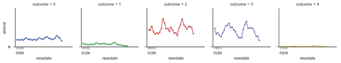
Outcome 0 is Return to Owner
Outcome 1 is Euthanasia
Outcome 2 is Adoption
Outcome 3 is Transfer
Outcome 4 is Died
We see that Numbers of animals euthanized declined starting in July 2015. Adoption rates seem to show a pattern of high and low rates. Death rates remain flat but low in Austin.
But doing a seasonality decomposition indicates some seasonality in adoption cycles.
adoption = (pvt1.loc[(pvt1['outcome'] == 2)])
s = (adoption[['year', 'animal']]).set_index('year')
series = s
result = seasonal_decompose(series,
model='multiplicative')
fig = plt.figure()
fig = result.plot()
fig.set_size_inches(8, 6)
plt.show()
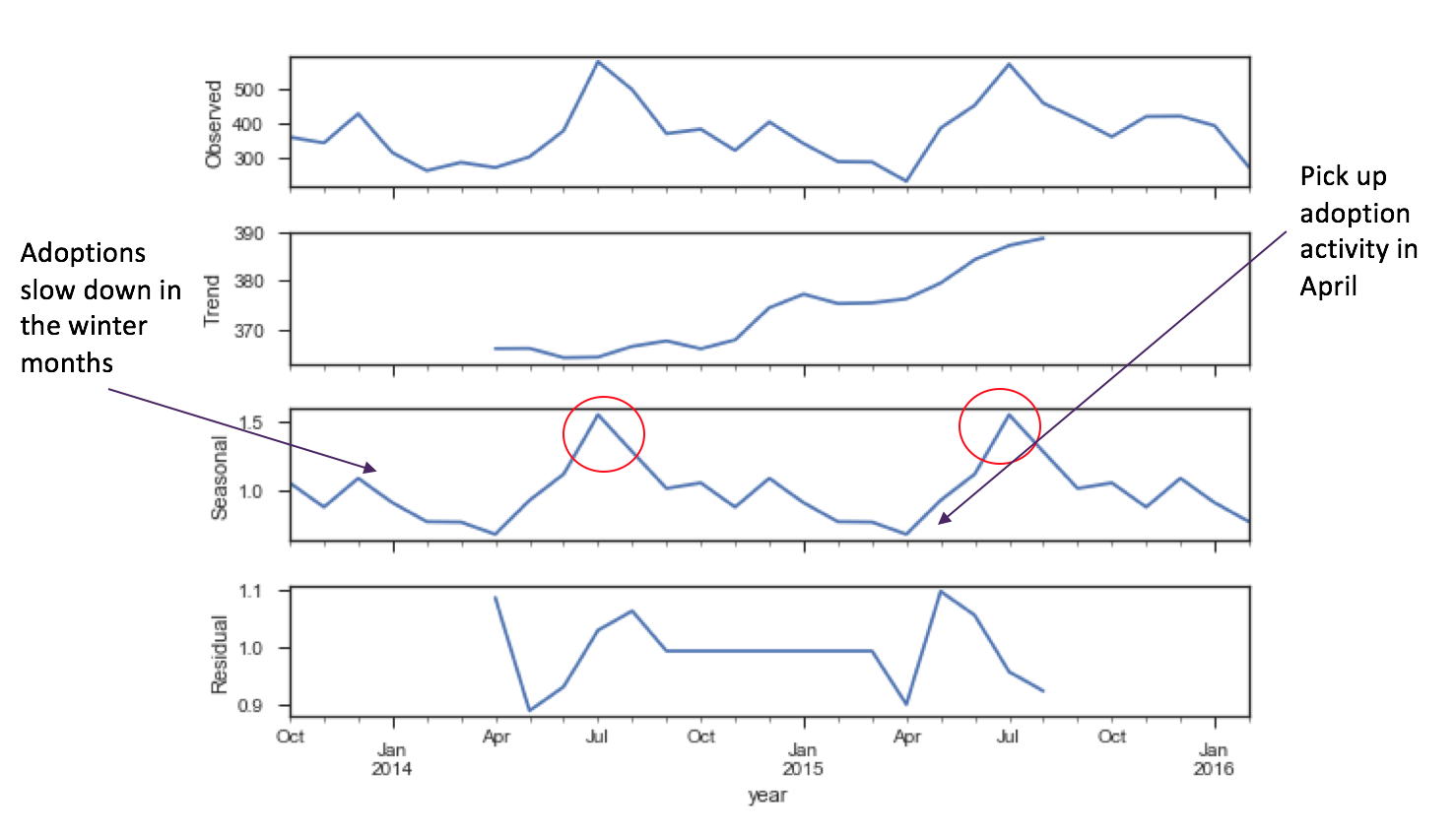
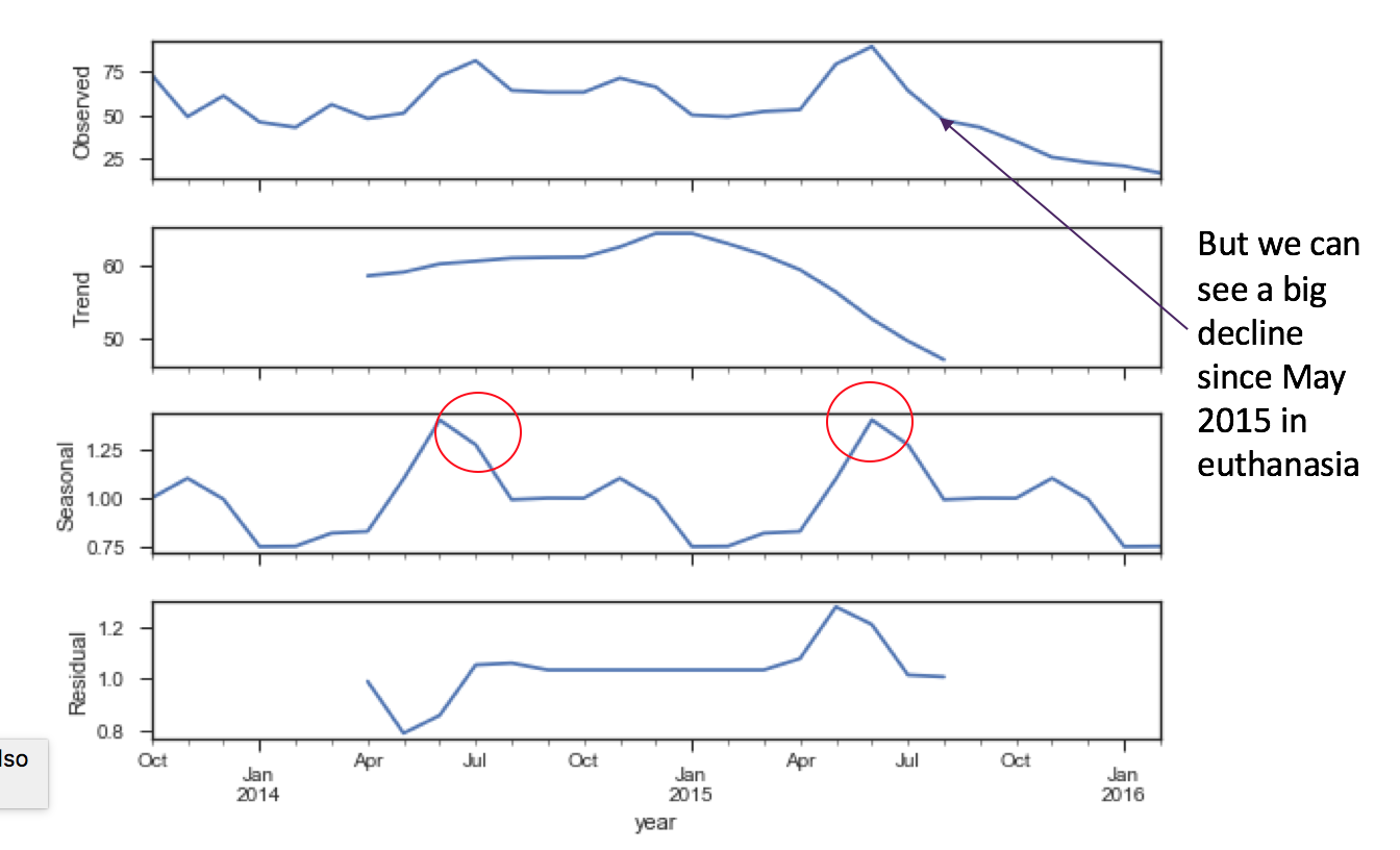
It makes sense to me that as the spring brings on nicer weather, more adoption events bring out people to adopt animals. Adoptions decline in the winter - maybe the shelter needs to do an adoption event to dress up dogs and cats in Santa Claus costumes to drive more adoptions? Certain policy interventions can help drive these trends in the future towards more positive cycles, if they choose to. Also, found that euthanasia peaks in the summer as well. Maybe people are mistreating animals over the winter months, and as the animals come in, they're in poor condition? Maybe there's an overcrowding condition. It is good to see however, that euthanasia rates decreased in the latter half of the final calendar year of this data.
euth = (pvt1.loc[(pvt1['outcome'] == 1)])
e = (euth[['year', 'animal']]).set_index('year')
series = e
result = seasonal_decompose(series,
model='multiplicative')
fig = plt.figure()
fig = result.plot()
fig.set_size_inches(8, 6)
plt.show()
Predict Animal Outcomes
Based on traits of the animal and the facility, we want to predict if the animal will have a 0 to 4 outcome, such as Outcome 2: Adoption. For this, I'll create a Random Forest Classifier.
X and y are purely using the data from the training set, that's split 70/30. Here's what we're doing as a cheat sheet:
Date datetime64[ns] - DROP
Age_Mos float64
outcome int64 - DROP (TARGET)
subtype int64
animal int64
sex int64
breed int64
color int64
name_ int64
year datetime64[ns] - DROP
year_fx int64
data = train_fin.copy()

#I want to use the month and year and use the year of adoption as a feature, too.

data['year'] = data.Date.map(lambda x: x.strftime('%Y-%m'))
data['year'] =  pd.to_datetime(data['year'])
data['year_fx'] = pd.factorize(data['year'])[0]


X = (data.drop(['outcome', 'Date', 'year'], axis=1)).values
y = data['outcome'].values

#random forest, do a 2/3, 1/3 split
X_train, X_test, y_train, y_test = sklearn.cross_validation.train_test_split(X, y,
test_size=0.30, random_state=0)
print(X_train.shape, y_train.shape)
print(X_test.shape, y_test.shape)
Here's what we're going to do:
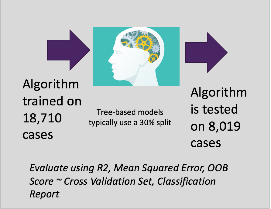
Let's get to a benchmark quickly.
clf = RandomForestClassifier(n_estimators=100, oob_score=True, random_state=42)

clf.fit(X_train, y_train)

#this is the r2 score
print(clf.oob_score_)

#feature importance
clf.feature_importances_
x_df = (data.drop(['outcome', 'Date', 'year'], axis=1))

feature_importances = pd.Series(clf.feature_importances_, index=x_df.columns)
feature_importances.sort()
feature_importances.plot(kind='barh', figsize=(6,3))
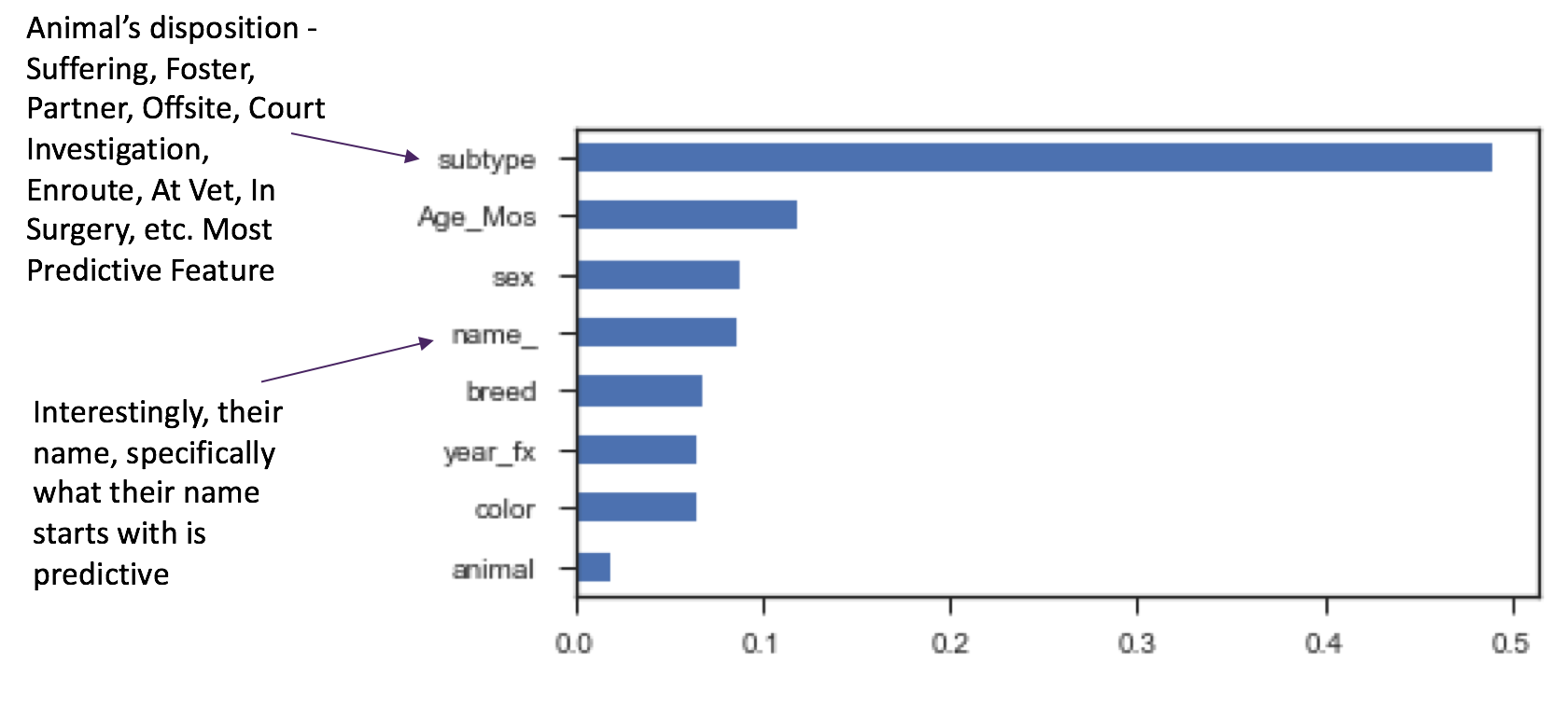
Feature importance indicates that the animal's disposition called 'subtype' is the most predictive for outcome. This makes sense, since these situations are also sub-types of the outcome. It may be even be a little biased, driving up our accuracy, since these are in fact, probably groupings of outcomes. Worth predicting for this subtype as another round of modeling.
What else is interesting is that the name of the animal, here indicated by the first character of the animal's name like "d" for "Dexter" or "m" for "Minnie" is predictive. At another round of modeling, I'd also drop the 'animal' feature, as there are only two animals in this set - dog or cat, and that doesn't appear as important as I had thought, in predicting the animal's outcome.
At this point, I applied some code that I learned from watching this very well narrated video on the Tutorial classification by Mike Bernico.
results = []
max_features_options = ["auto", None, "sqrt", "log2", 0.9, 0.2]
for max_features in max_features_options:
model = RandomForestClassifier(n_estimators = 500, oob_score=True, n_jobs=1, random_state=42, max_features = max_features)
model.fit(X,y)
print(max_features, "option")
score = model.oob_score_
print("r2", score)
results.append(score)
print("")
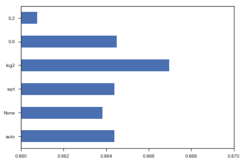
pd.Series(results, max_features_options).plot(kind='barh', xlim = (.86, .87));
#min_samples_leaf - the minimum number of samples in newly created leaves
results = []
min_samples_leaf_options = [1,2,3,4,5,6,7,8,9,10]
for min_samples in min_samples_leaf_options:
model = RandomForestClassifier(n_estimators = 500, oob_score=True, n_jobs=1, random_state=42,
max_features = 'log2')
model.fit(X,y)
print(min_samples, "min samples")
score = model.oob_score_
print("r2", score)
results.append(score)
print("")
pd.Series(results, min_samples_leaf_options).plot(kind='barh', xlim = (.863, .867));
The outcome of which, led me to fit this final Random Forest Classifier with an r2 of 0.866960978712.
#Final Model

clf = RandomForestClassifier(n_estimators = 500,
                         oob_score=True,
                         n_jobs=-1,
                         random_state=42,
                         max_features = 'log2')
clf.fit(X,y)
score = clf.oob_score_
print("r2", score)
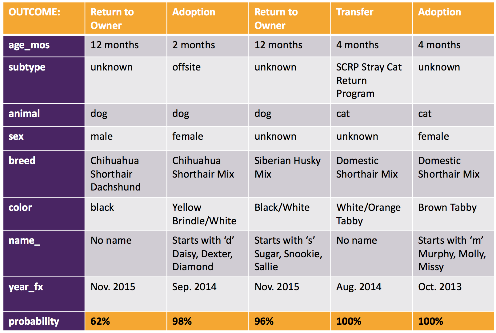
Here are the outcomes predicted for a sample of 5 of the 8,106 test cases:
We can also compare different models based on the hyperparameters we optimize. In this case, as we add more trees – called ‘estimators’ – our error goes down using the blue model – that’s the one I chose.
In this example, I chose to evaluate the error for max_features 'sqrt', 'log2', and 'auto', using code from scikit learn:
ensemble_clfs = [
("RandomForestClassifier, max_features='sqrt'",
    RandomForestClassifier(warm_start=True, oob_score=True, max_features='sqrt')),
("RandomForestClassifier, max_features='log2'",
    RandomForestClassifier(warm_start=True, max_features='log2', oob_score=True)),
("RandomForestClassifier, max_features='auto'",
    RandomForestClassifier(warm_start=True, max_features='auto', oob_score=True))]

# Map a classifier name to a list of (<n_estimators>, <error rate>) pairs.

error_rate = OrderedDict((label, []) for label, _ in ensemble_clfs)

# Range of `n_estimators` values to explore.

min_estimators = 15
max_estimators = 175

for label, clf in ensemble_clfs:
    for i in range(min_estimators, max_estimators + 1):
      clf.set_params(n_estimators=i)
      clf.fit(X, y)

# Record the OOB error for each `n_estimators=i` setting.
oob_error = 1 - clf.oob_score_error_rate[label].append((i, oob_error))

# Generate the "OOB error rate" vs. "n_estimators" plot.
for label, clf_err in error_rate.items():
   xs, ys = zip(*clf_err)
   plt.plot(xs, ys, label=label)

plt.xlim(min_estimators, max_estimators)
plt.xlabel("n_estimators")
plt.ylabel("OOB error rate")
plt.legend(loc="upper right")
plt.show()
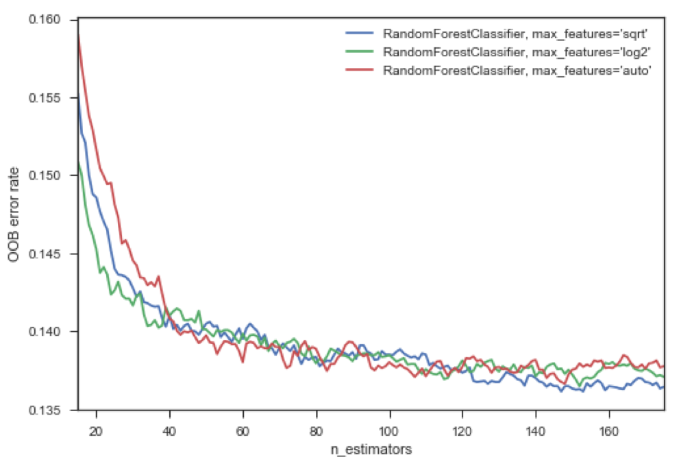
We can see that the blue curve which is the model I ran, using the 'log2' parameter indicates with increasing number of estimators, a reduced OOB error rate compared to its green and red peers.
Next Steps?
What I would do to revisit this model is elaborate on the time series model by conducting a time series forecasting model based on not the 0 - 4 outcomes, but also by the subtypes - remember, those 'foster', or 'suffering' conditions associated with the outcome.
I'm also curious about the features like name. I'd explore the predictions on the test set to understand which animal name types - ones that start with D or start with M? are more successful to be adopted, or worse-off, euthanized.
I'd also run the model again by dropping the 'animal' variable, since at first glance it seems that the nature of being a dog or cat doesn't influence the outcome.
For the purpose of the 15-minute presentation, I think this project provided a good basic overview of what machine learning prediction can do.