Amazon Food Reviews, Part I
It takes time to take advantage of all the great data science/ML resources out there like Coursera, Udacity, HackerRank, and Kaggle competitions. I won't bore you with the details, but granted that life sometimes gets in the way, one of my goals is to get into Kaggle a bit more.
Over the weekend I finally set up a Kaggle account and downloaded this awesome data set: Amazon Fine Food Reviews. After opening "Reviews.csv", I decided to do a few things:
- Apply the TextBlob sentiment analyzer to each of the 568,454 reviews and explore how it and some other interesting features changed over the past 5 years
- Analyze what is the distribution of reviews and products that are perfectly positive and perfectly negative in sentiment?
- Return the Top 50 features for perfectly positive sentiment reviews, when the user enters a Score (1 to 5).
- Return trigrams for comments where the polarity sentiment is 1.0 positive and Score = 5, and when -1.0 negative and Score = 1
- Predict the Score based on a user entering an Amazon Review using a Naive Bayes classifier.
Sentiment Analysis
Today we'll embark on Task 1: Using out-of-the-box TextBlob to analyze the sentiment for each of the reviews, and analyzing the metrics over the past five years.First, we need to read in the data and clean it using BeautifulSoup: After briefly skimming through the dataframe, it didn't seem like there were text encoding issues, but thought it would be safer to run bs4 anyway
from __future__ import division
from __future__ import print_function
import nltk
import pandas as pd
import numpy as np
import matplotlib.pyplot as plt
import seaborn as sns
import pylab
from bs4 import BeautifulSoup
import textblob
from textblob import TextBlob
import pickle
import datetime
from scipy.stats import kendalltau
data = pd.read_csv("/...amazon-fine-foods/Reviews.csv")
print(data.dtypes)
#clean text using bs4 - approx. 10 minutes
data['text_cln']= data['Text'].map(lambda x: BeautifulSoup(x, "lxml").get_text())

#apply the polarity score to each text feature using
TextBlob (took approx 5 minutes)

data['tb_polarity']= data['text_cln'].map(lambda x:
TextBlob(x).sentiment.polarity)

#pickle
data.to_pickle('amz_data.pkl')
#read pickle
dir_name = ".../data"
data = pd.read_pickle('amz_data.pkl')

#normalize date time
data2 = data.copy()
data2['datetime'] = data2['Time'].map(lambda x: (datetime.datetime.fromtimestamp(int(x)).strftime('%Y-%m-%d %H:%M:%S')))
data2['datetime'] = pd.to_datetime(data2['datetime'])
Check out the data
print(data2.dtypes)
print(data2.describe())
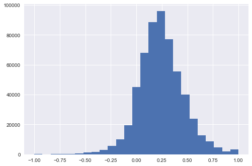
#distribution of tb_polarity, mean = 0.241566
data2['tb_polarity'].hist(bins=25)
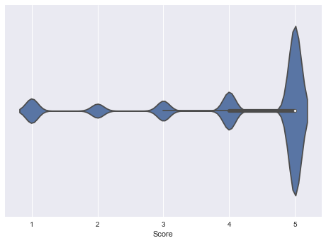
#violin plot for distribution of each 5 scores
sns.violinplot(data2['Score'])
At this point I'm interested in learning how not only the polarity sentiment score, but how the other features change over time, specifically year-to-year from 2008 to 2012.
timecopy = data2.copy()
timecopy.set_index('datetime', inplace=True)
At this point, "cut" different frames by specifying a start and end calendar date. For each df, create a series that indicates the sentiment (polarity) mean, the Score mean, the Helpfulness Numerator and Denominator means, the number of comments for that year, and the number of unique products (as specified by the Product Id variable):
time2012 = timecopy.loc['2012-1-01':'2012-12-31']
s1 = [time2012['tb_polarity'].mean(),
time2012['Score'].mean(),
time2012['HelpfulnessNumerator'].mean(),
time2012['HelpfulnessDenominator'].mean(),
len(time2012),time2012['ProductId'].nunique()]

time2011 = timecopy.loc['2011-1-01':'2011-12-31']
s2 = [time2011['tb_polarity'].mean(),
time2011['Score'].mean(),
time2011['HelpfulnessNumerator'].mean(),
time2011['HelpfulnessDenominator'].mean(), len(time2011),
time2011['ProductId'].nunique()]

time2010 = timecopy.loc['2010-1-01':'2010-12-31']
s3 = [time2010['tb_polarity'].mean(),
time2010['Score'].mean(),
time2010['HelpfulnessNumerator'].mean(),
time2010['HelpfulnessDenominator'].mean(), len(time2010),
time2010['ProductId'].nunique()]

time2009 = timecopy.loc['2009-1-01':'2009-12-31']
s4 = [time2009['tb_polarity'].mean(),
time2009['Score'].mean(),
time2009['HelpfulnessNumerator'].mean(),
time2009['HelpfulnessDenominator'].mean(), len(time2009),
time2009['ProductId'].nunique()]

time2008 = timecopy.loc['2008-1-01':'2008-12-31']
sns.violinplot(time2008['tb_polarity'])
s5 = [time2008['tb_polarity'].mean(),
time2008['Score'].mean(),
time2008['HelpfulnessNumerator'].mean(),
time2008['HelpfulnessDenominator'].mean(), len(time2008),
time2008['ProductId'].nunique()]
Now create a dataframe with s1, s2, s3, s4, and s5 loaded:
df = pd.DataFrame([s5,s4, s3, s2, s1], index=['2008', '2009', '2010', '2011', '2012'], columns =['mean polarity', 'mean Score', 'mean HNum', 'mean HDen', 'count', 'num_products'])
Plot the distributions of:
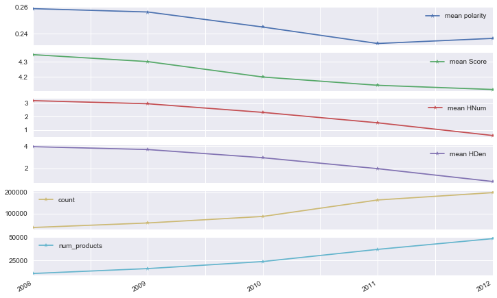
Since 2008, it looks like the the sentiment of each review has decreased slightly, hitting a low point in 2011. Also in 2011, the Score and Helpfulness metrics reached a low. But, it's also worth noting that the data shows the number of products have been increasing steadily, around 30% year over year. From 2008 to 2012, we see a 4.5 fold increase in the number of products. It's hard to tell whether the increase in products offered at Amazon also led to customers reviewing products in a more scrutinized fashion as well, leading to lower sentiment and score ratings.
What may help as a next step in a follow-up post is to do a chi-square year-to-year, to measure the statistical significance of the sentiment and scores.
Here's the rub:
I've used the TextBlob sentiment polarity score about a few dozen times now and almost all the time the mean centers around the 0.20-ish range. Here we see the same thing for the entire corpus for all years (mean = 0.241566). Is polarity a metric that helps us better understand the reviews? Well, in doing a spearman correlation between 'tb_polarity' and 'Score', it was only 0.426811 meaning that polarity explains only (0.426811^2 = 18%) of the Score. So overall polarity is probably a weak measure. (Spearman: 0.40293056470670224, Kendalltau: 0.31643791593598869) Or it could be that this particular way of measuring polarity isn't good enough, and it requires us to build our own classifier. Alternatively, I could implement on the second time around, the Naive Bayes or Decision Tree classifier available in TextBlob that simply categorizes a review as positive or negative.